Histograms are used to summarize discrete or continuous data. In other words, it provides a display of numerical data by showing the number of data points that are within a certain range of values ​​(called “bins”). 

This is similar to a vertical bar chart. However, a histogram, unlike a vertical bar chart, does not show any gaps between the bars.

What is a histogram?

Histograms are a way to display the number of data and are similar to bar charts. The bar chart shows the actual number against the categories; The height of the bar indicates the number of items in that category. The histogram displays batch variables in “bins”.

A class indicates how much data is in a range. Usually, a range is selected that best fits the information. There is no rule for the number of floors, but as a rule, 5-20 floors is good.

If you select more than 20 layers, reading the chart will be difficult and complicated, and less than 5 histograms will have no specific message or meaning. Most charts that are created on a basic scale have about 5 to 7 buckets.

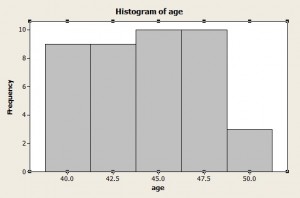
Graph with 5 floors

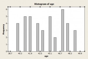
Graph with high number of classes

Another rule of thumb is that if a value falls into two ranges, place it in the upper range. For example, if he has a histogram of ages and the distances are between 42-40 and 44-42, a person who is 42 years old should be between 44-42.

 

What is the height of the bar in the histogram?

Unlike a bar chart, the area of ​​a range in a histogram represents its frequency, not its height. This frequency is calculated by multiplying the width of the range by the height. The height of the bar in the histogram indicates the frequency (number) only if the width of the ranges is equal.

For example, if you draw a large amount of earthquake and the ranges are 3-5, 7-5 and 7-9, the height of the bar is equal to the frequency (number). However, histograms do not always have the same distances. When the histogram has uneven distances, the height is not equal to the frequency.

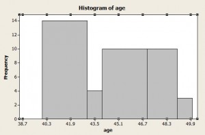
Histogram with uneven distances (height does not indicate frequency)

Bihistogram

A bihistogram is a graph made up of two histograms (“bi” = two) in opposite directions. One histogram is above the axis and one is below. Histograms can be either y-axis or x-axis. Each direction represents a different category.

Bihistogram is a visual alternative to independent t-test and can be more useful than t-test because many features are seen in the chart, such as:

• Integrity
• Location (where the horizontal axis is the focus chart)
• Scale (if the graph is drawn or compressed)
• Drop data

Making a Bihistogram

Bihistogram is rarely used compared to other statistical techniques, so most popular software does not have the ability to create it. This diagram can be drawn in both R and Dataplot software. SPSS software also provides a tool that can be used to put histograms together.

Bihistogram in R

There is no simple function in R to create a Bihistogram, but StrictlyStat suggests stacking two histograms on top of each other.

Dataplot

The Dataplot uses the BIHISTOGRAM command.

Bihistogram in SPSS 20

1. Click on “Graphics” in the menu, then select “Chart Builder”.

2. Select the histogram from the gallery on the left and bottom. A set of different histograms appear.

3- Drag and drop the desired chart to the preview area (drag).

4. Select the variable you want to draw the histogram (from the Groups / Point ID section) and drag and drop it on the chart (drag).

Histogram Construction: An Overview

A histogram is a graphical representation of a group of numbers according to how they appear. This article will teach you how to make a histogram diagram by hand, but it is best to do this using other technologies, such as Excel.

The choice of ranges in statistics is usually a matter of empirical estimation. When you do the histogram by hand, you have trouble choosing the ranges. Using Excel (other software), after creating a histogram, you can change the ranges until you find the chart you want.

Sometimes you have to make a histogram by hand, especially if you have a relative frequency histogram; Technology like the TI-83 only creates a regular frequency histogram. If you have to make a histogram by hand, here is an easy way to explain it.

Histogram construction: steps

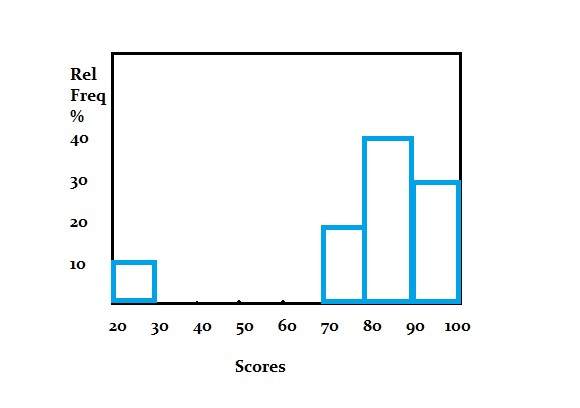
Sample question: Make a histogram for the following scores:

99, 97, 94, 88, 84, 81, 80, 77, 71, 25

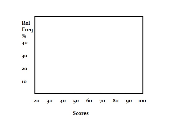
Step 1: Draw the X and Y axes. For example, the X axis is labeled “score” and the Y axis is labeled “relative frequency percentage”.

Step 2: Select the number of intervals and label the chart. In this example, 10 intervals (the X axis is the interval) are a good choice (you seem to have 5 bars with one or two items in each group).

Step 3: Divide 100 by the number of data points to get the idea of ​​where to put the frequency. There are 10 items in the dataset, so that means% 10 = 10/100 (one item equals 10% of the total).

Step 4: Count the number of items in each interval and then draw a rectangle on the chart that corresponds to the percentage of the total interval. In this sample data set, the first interval (20-20) has 1 item, (80-70) has two items. If an item is in the range range (for example, 80), place it in the next range (90-80).

Notes

Tip 1: If you are unsure about how many times to select an interval, create an online chart using Shodor.org. Change the intervals until you reach the desired chart.

Tip 2: Choosing a place to place a frequency tick is also somewhat arbitrary and rarely scientific. For example, if you have 21 items, you can set the tick to 5%, although each number is slightly less than 5%. Keep this in mind when designing the chart.

Warning: Selecting the optimal interval size is complicated in large datasets. It is better to use technology for large data sets.

How to build a histogram in Minitab

Minitab is software that is similar to Excel and other spreadsheet programs.

How to build a histogram in Minitab: Steps

Step 1: Enter your information into the columns in Minitab. In most histograms, you will have two sets of variables in two columns.

Step 2: Click on “Graph” and then click on “Histogram”.

Step 3: Select the type of histogram you want. In most cases, a “simple” histogram is usually the best option for basic statistics.

Step 4: Click “OK”.

Step 5: Select the name of the variable for which you want to create a histogram, and then click the “Select” button to move the variable name to the graph variables box.

Step 6: Click OK to create a histogram in Minitab.

Step 7: (Optional) Change the number of intervals (handle width) by clicking on one of the binary rows (numbers) at the base of the bar. This box opens the edit box. Click “Binning” and then the “Number of intervals” button. Change the number of intervals and click “OK”.

Note: When entering data into Minitab, be sure to enter the names of the significant variables in the first row (column header). This makes it easier to select the variable in step 5.

 

How to build a histogram in SPSS: Steps

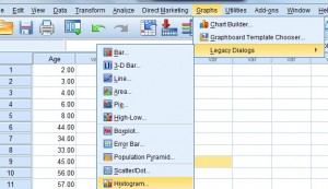
Step 1: Click on “Graphs”, then click on “Legacy Dialogs” and select “Histogram…”.

Step 2: Select one of the variables from the dialog box on the left and then click on the center arrow to move your selection to the “Variable” box.

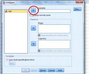
Step 3: Click “OK”. SPSS takes a few moments to create a chart. In the meantime, you will see a blank page with the words “Running Graph” at the bottom right.

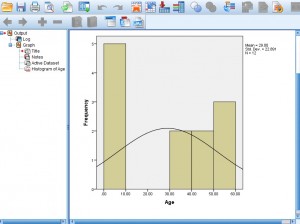
Note: To edit the scales, height, width and other features of the SPSS histogram, double-click on the output chart (this is the window that opens with the chart) and then double-click on the feature you want.

Note: If you want the data to have a normal distribution, check the “Display Normal Curve” box.

Warning: Histograms work with a set of variables using this method, so do not try to select more than one variable at a time. If you need more than one histogram for a set of different variables, repeat the steps above. SPSS opens a new window with each histogram.

Histogram on TI-83: ​​Overview

Suppose you have a list of the tallest buildings in New York. Here’s how to put it on the TI-83 and convert it to a histogram.

Histogram TI-83: ​​Steps

Example Problem: Draw a histogram showing 20 tall buildings in New York. The height of 20 buildings (in feet) are: 1250, 1200, 1046, 1046, 952, 927, 915, 861, 850, 814, 813, 809, 808, 806, 792, 778, 757, 755, 752 and 750.

Step 1: Enter the data into the list. Press the STAT button and then press ENTER for the “Edit” option. Enter the first number (1250) and press ENTER. Continue entering the numbers, press the ENTER button after each number.

Step 2: Press “2nd”, then select “Y =” equal to “Stat Plot”.

Step 3: Press “ENTER” to select the design.

Step 4: Press ENTER again. This option selects “On”.

Step 5: Look at the down arrow key (arrow keys are on the top right), then press the right arrow button twice. The cursor should flash on the histogram option at the top right of the list.

Step 6: Scroll to the bottom of XList and enter the name of the list where you entered your data in step 1. If this is the first time you have created a list, you are likely to enter “L1”, which is the default list. If “L1” is not displayed, press “2nd” and then press “1” to select “L1”.

Step 7: Scroll down and then type “1” for “Freq”.

Step 8: Press the “Graph” button. The histogram is displayed on the screen. Press “Zoom” and then “Zoomstat” to view the histogram.

Notes

Tip 1: Press the TRACE button and with the front and back or left and right buttons, the number of items in each group (n =) as well as the top and bottom class restrictions will be displayed.

Tip 2: To change the class width, press WINDOW and change Xscl. For example, if you want to set the class width to 100, (probably the most suitable for the above data) change “Xscl” to “100”.

This is how to create a histogram in TI-83!

Example 2

Draw a histogram for the following scores in a statistics class:

45, 67, 68, 69, 74, 76, 75, 77, 79, 84, 86, 90%.

Step 1: Press STAT, then press ENTER to edit L1.

Step 2: Enter the data into the list. Press ENTER after each entry. For example, for the first two inputs you can type:

ENTER 5 4

ENTER 7 6

Step 3: To access the Stat Plot menu, press 2nd and then Y =.

Step 4: Press ENTER twice to turn on Plot1.

Step 5: Go to Type which has 6 icons to the right. Select the upper right icon that looks like a histogram with ENTER.

Step 6: Make sure the XList “” input reads L1. If he did not read L1, hit Clear, then 2nd and 1.

Step 7: Click on Graph. You should see a histogram.

Notes

Note: When you tap Graph, if you see the message “Err: Stat” or the histogram you were expecting, then press “Window” and try different settings. Especially if you try to change the Xscl (X Scale) to a larger value.

Histogram TI-89

When you enter and chart your data for the TI-89 histogram, the TI-89 even counts the number of items in each bar (class).

Histogram TI 89: Steps

Example Problem: Create a histogram for car costs: 12500; 22400; 14300; 32200; 21,500; 1980; 15001; 22001; 32036; 35124; 29001; 25006; 27001; And 18500.

Step 1: Press APPS and go to the Stats / List editor. Press ENTER.

Step 2: First press F1 and then 8 to clear the data list editor.

Step 3: Enter “cars” as the list name by pressing 2nd ALPHA = 23 ENTER.

Step 4: Enter the information:

ENTER12500

ENTER22400

ENTER14300

ENTER32200

ENTER21500

ENTER19980

ENTER15001

ENTER22001

ENTER32036

ENTER35124

ENTER29001

ENTER25006

ENTER27001

ENTER18500

Step 5: First press F2 and then ENTER and go to Setup Plot (Define Plot) by pressing F1.

Step 6: Press the scroll arrow to the right to create a menu for the Plot Type. Press 4 for the histogram.

Step 7: Press the down arrow “x” then press 2nd – (minus key) to raise Var-Link. Go to “cars” and press ENTER.

Step 8: Scroll down to Hist. Select Bucket Width and enter 5000 and then press ENTER. This is the width of your class.

Step 9: Press ENTER and F5. Note: If you press ENTER several times and the home screen is finished, press the diamond key and then F3 (to draw a chart).

Step 10: Press 3 to track performance. Use the left and right scroll keys to move from one bar to another. (It will tell you how many items are in each class. (N = x)).

 

Notes

Tip 1: If the TI 89 histogram is not displayed (only part of the chart is shown), you may need to change the window. Press the Diamond key and then press F2 to check your window settings. For the above diagram, the settings should be approximately equal to x <40000> 10000 and 0 <y <8. Set xscl and yscl to 1. Press F2 and then 9 to return to the chart.

Tip 2: Make sure the alpha lock is on. By checking a small black box with an “a” at the bottom left of the screen.