


What Is A Decision Tree In Machine Learning And What Is Its Application?
A Decision Tree, Or Simply A Decision Tree, Is A Way To Show The Decision-Making Process Through A Tree Structure.
The decision tree is typically used for planning and defining operational business decisions through visual diagrams (Visual Flowchart).
What a decision tree does is that it represents a branch of decisions where the end of each chapter points to the outcome. Each tree branch is a structure or representation that refers to different choices to choose the most desirable and optimal solution finally.
The decision tree is included in the classification and regression methods. Decision trees are significant in programming and computer networks because they provide optimal and accurate solutions to problems.
The point we should mention about the decision tree is that the above concept has existed for several decades and was previously brought to the attention of programmers through a concept called flowcharting.
Also, economic experts use decision trees in business operations, economics, and operations management to analyze organizational decisions.
What is a decision tree?
The decision Tree Algorithm is a popular supervised machine learning algorithm suitable for working with complex data sets due to its straightforward approach. The reason for naming decision trees is their functional similarity to a tree’s roots, branches, and leaves, which shows themselves in the form of nodes and edges. They are similar to flowcharts for analyzing decisions based on the “what if” pattern. The tree learns these if-else decision rules to partition the data set to create a tree model.
Decision trees are widely used in predicting discrete outcomes, classification problems, and continuous numerical outcomes for regression problems. Various algorithms exist in this field, including CART, C4.5, and ensembles such as random forests and gradient-enhanced trees.
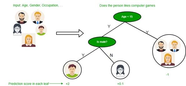
Decision tree algorithms are classified under supervised learning and can be used to solve regression and classification problems. A decision tree uses a tree representation to solve this problem, where each leaf node corresponds to a class label, and features are represented in the inner node of the tree. We can define any Boolean function on discrete components using a decision tree. The figure below shows this problem.
At first, we consider the entire educational set as the root.
We add attribute values that are more valuable to the category. In this case, if the values are continuous, they are discrete before building the model.
Based on attribute values, records are recursively distributed.
We use statistical methods to sort attributes as roots or internal nodes.
Application of decision tree in the field of machine learning
As mentioned, a decision tree is a mechanism for shaping or organizing an algorithm that is supposed to be used to build a machine learning model. The decision tree algorithm is used to divide the features of the data set using the cost function.
An important point to note is that the algorithm grows in a way that shows features unrelated to the problem before it takes action to optimize and remove extra branches. For this reason, pruning removes additional components, just like in the real world, where tree branches are pruned.
In the decision tree algorithm, it is possible to set parameters such as the depth of the decision tree so that the problems of overfitting and excessive complexity of the tree are minimized.
Today, various decision trees are used in machine learning for object classification problems based on the trained features.
Interestingly, machine learning programmers also use decision trees in regression problems or predicting continuous outcomes of unseen data. By providing a visual and understandable view, decision trees simplify the decision-making process and the process of developing machine learning models.
Accelerate The only negative thing about decision trees is that as the number of tree branches increases, the process of understanding and using them becomes difficult due to the excessive complexity of the tree; Hence, pruning is a technique that should be used for trees.
Generally, we should say that a decision tree is a structured solution for illustrating decisions, modeling them, and receiving detailed outputs to show the success rate of options (decisions) in achieving a specific goal.
Familiarity with some commonly used terms of decision trees
Before we examine the decision tree architecture, we must first mention some essential and widely used words in this field.
- Root Node: represents the problem data set divided into two or more homogeneous sets. The root node is the highest node of the decision tree.
- Splitting is a process of dividing nodes into two or more sub-nodes.
- Terminal Node: The terminal nodes of each branch, which cannot be divided, are called leaf nodes or terminal nodes.
- Pruning: In most cases, we must remove the redundant parts of a tree. When subnodes need to be removed from the decision node, the pruning process begins. In general, we must say that pruning is an operation opposite to separation.
- Sub-tree or branch (Branch / Sub-Tree): The subsections of the decision tree are called branches or sub-trees.
- Parent and Child Node: A node divided into other subnodes is called the parent node of the subnodes. In this case, the created nodes are the children of that parent node.
Figure 1 shows the concepts and terminology around the decision tree.
Decision trees have different nodes. The first node is called the root node, the starting point of the tree containing the problem data set. Next are the leaf nodes, the endpoints of each tree branch, or the final output of a set of decisions.
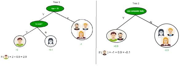
Each branch of the decision tree in the field of machine learning has only one leaf node so that the attribute of the data in the internal nodes of the components and their result in the leaf of each chapter are shown. Figure 2 shows a view of a decision tree.
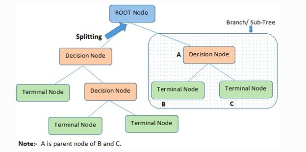
figure 1
As shown in Figure 2, decision trees help programmers find the most optimal solution by providing a simple and understandable visual view.
figure 2
One of the essential concepts related to the decision tree and machine learning is explainability. Explainability refers to the process of explaining the output of a model to technical and non-technical people. Fortunately, decision trees implement this process very well.
One of the most critical aspects of machine learning is the optimization of tasks without the direct intervention and control of experts; however, in most cases, it is difficult to explain the output and what a model does. For this reason, machine learning experts use the tree structure and branches of a tree to explain each decision machine learning makes.
How does the decision tree work?
Decision trees use several algorithms to decide whether to split a node into two or more sub-nodes. Decisions about strategic divisions strongly affect the accuracy and performance of the tree; that’s why classification and regression trees use different criteria to make decisions.
The decision tree divides the nodes based on the available variables. Also, decision trees use several algorithms to decide whether to split a node into two or more sub-nodes. Interestingly, the process of dividing and building sub-nodes increases their homogeneity. In other words, a node’s desired performance is directly related to the target variable (metric) used.
One thing you should pay attention to as a machine learning engineer is that the algorithm selection is based on the type of target variables.
Among the essential algorithms that can use in decision trees should be the following :
-
It’s a Decision Tree Algorithm (ID3), which some sources call Iterative Dichotomiser 3. The ID3 algorithm creates a multipath tree based on the greedy search approach and finds each node’s discrete and group features. ID3 algorithms in the field of machine learning provide the most information on problems that are based on discrete objectives. As the name suggests, a greedy algorithm always makes the choice that seems best at that moment.
-
Another widely used algorithm is decision tree C4.5, which replaced ID3. The above algorithm provides a dynamic definition for a discrete feature based on numerical variables that divide the continuous feature values into a set of discrete parts; So that they remove the limitation around the elements that should have a discrete state.
-
The CART decision tree algorithm, which some sources call classification and regression trees, is very similar to the C4.5 algorithm. The difference between the above two algorithms is that the CART algorithm supports continuous and numerical target variables and does not perform any calculations on the rules. To be more precise, the algorithm creates a binary tree through the feature and threshold that makes the most data set in a node.
-
In each step, the CHAID decision tree algorithm, which some sources call the Chi-squared Automatic Interaction Detection algorithm, uses the predictor variable that interacts most with the dependent variable in constructing the tree. The above algorithm uses chi-2 when calculating and dividing multilevel trees. May combine Levels of classes of each predictor variable to create an understandable level.
-
MARS Decision Tree Algorithm, or Multivariate Adaptive Regression, is an algorithm used to solve complex nonlinear regression problems. This algorithm searches through a set of simple linear functions to provide the best performance for predictions.
The calculation process starts from the root node in the decision tree to predict the desired classes of the problem data set. The binary algorithm compares the data feature value with other subnodes for the next node and continues the tree-building process. This process continues until the tree’s leaf node or end node is reached. In this case, the algorithm compares the values of the root attributes with the data attributes, follows the branches, and goes to the next node based on this comparison.
The process of performing these processes step by step is as follows:
- First step: The decision tree algorithm starts from the root node based on all the data.
- Second step: The ideal feature in the data set is selected based on the Attribute Selection Measure (ASM) mechanism.
- The third step is dividing the root node into subsets that will include ideal values or the best features.
- The fourth step: is the process of making a node that has precise characteristics.
- Fifth step: new decision trees are created reverse Based on the designed subsets. This process continues until it is impossible to categorize and divide the nodes. The final node is considered a leaf or terminal node in this case.
For example, suppose a person has a job offer and intends to choose or reject this job position based on his assumptions.
If this problem is to be solved based on a decision tree, the process of doing things is as follows:
The decision tree algorithm starts with the root node and salary attribute based on the measurement of that attribute. Next, the root node is divided into the next decision node, the node related to the distance from the office, and a leaf node based on the relevant tags to reject the job offer request.
Next, decision-making nodes are divided into organization facilities and job offer rejection nodes. Finally, the decision node is divided into two leaf nodes, i.e., Accepted offers and Declined offers. Figure 3 shows building a tree based on the explanations we provided.
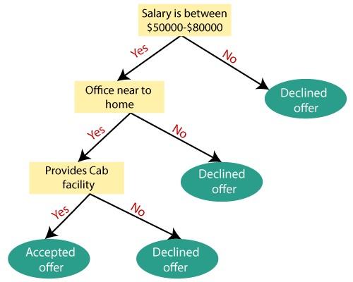
Figure 3
Attribute Selection Measures
When designing and implementing a decision tree, an important issue is choosing the best feature for the root node and child nodes. A solution called “Attribute Selection Measure” is used for this problem. The feature selection measurement method is implemented based on two techniques: the above process can select the best feature for the root node and other tree nodes.
- Information Gain
- Gini Index
What is information acquisition?
Information acquisition means collecting data by measuring variation along with impurity (entropy) after partitioning a data set based on features. When we use a node in a decision tree to divide the training samples into smaller subsets, the entropy will Change. The increase in information is a measure of this change in entropy. The above method evaluates how much information a feature has about a class. Based on the obtained values, the process of dividing the nodes is done, and the decision tree is built. The decision tree algorithm always tries to get the most information. Next, it divides the node that has the most information. In the above method, information is obtained based on the following formula:
Information Gain= Entropy(S)- [(Weighted Avg) *Entropy(each feature)
Entropy is a measure of impurity in a given feature that also characterizes the randomness of the data. Entropy measures the uncertainty of a random variable, the impurity of an arbitrary set of examples. The higher the entropy, the higher the information content. The above criterion is calculated based on the following formula:
Entropy(s)= -P(yes)log2 P(yes)- P(no) log2 P(no)
- In the formula above, S is the number of all samples.
- P(yes): indicates the probability of a positive answer.
- P(no): indicates the probability of a negative answer.
When you intend to build a decision tree using information, you should pay attention to the following:
Start with all the training examples associated with the root node.
Use the information obtained to select a feature to label each node. Note that no root-to-leaf path should have the same discrete property twice.
Construct each subtree recursively on the subset of training samples classified in the tree.
If all training examples remain positive or negative, a label that node as “yes” or “no” accordingly.
If no features remain, label the training examples remaining at that node.
And if there are no examples left, label the parent training examples.
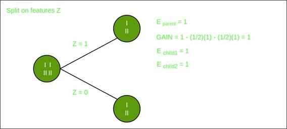
Now, let’s draw a decision tree for the following data using the Information gain method.
Educational set: 3 features and two classes
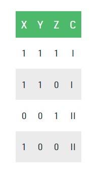
Here, we have three properties and two output classes that we used the information obtained to construct. We get each feature and calculate the information about each element.
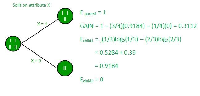
Division on feature X
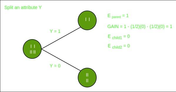
Division on the Y feature
What is the Gini index?
The Gini index measures the number of times a random element is incorrectly identified in the data set obtained when constructing a decision tree with the CART algorithm. This index is only used to create a class and binary groups. The decision tree should select the feature with the lowest Gini index value in this case. The Gini index is calculated based on the following formula:
Gini Index= 1- ∑jPj2
Consider the data set in the figure below to draw a decision tree using the Gini index.
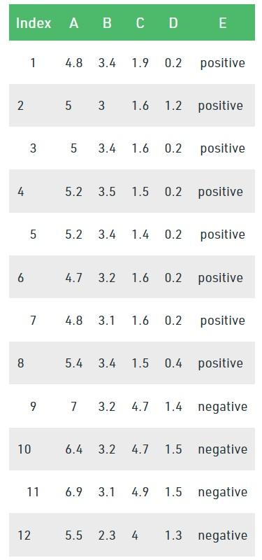
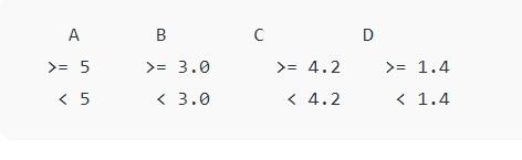
In the above data set, there are five features, and feature E is the predictive feature that includes two classes (positive and negative). We have an equal ratio for both types. We need to choose random values to categorize each component in the Gini index. These values for this data set are:
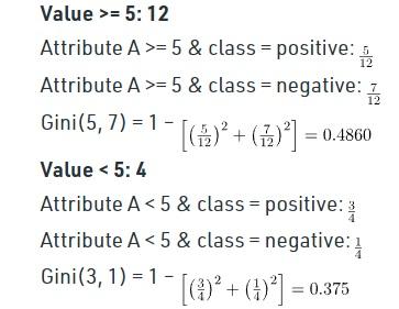
The calculation of the Gini index for A is as follows:
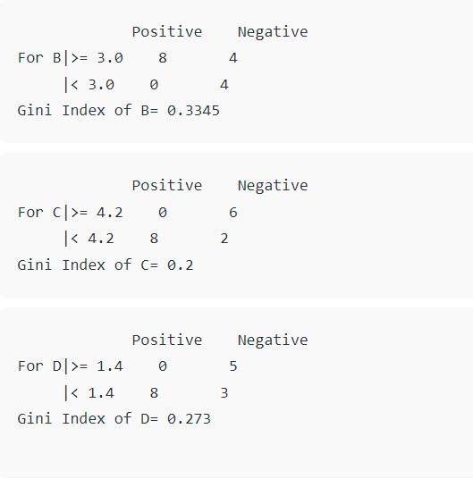
The analysis of the Gini index for B is as follows:
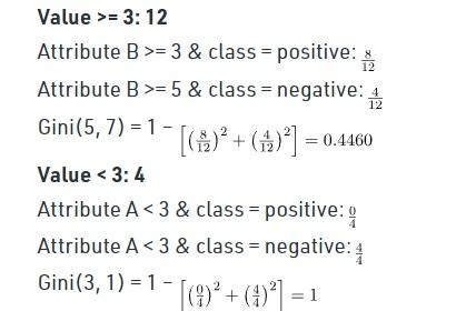
And the study of the Gini index for C and D are as follows:
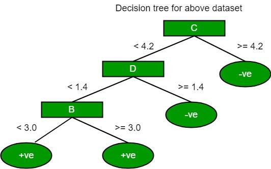
Now the above tree is as follows:
What is a decision tree return binary splitting?
Building a binary decision tree is a process of partitioning the input space. A greedy approach to space partitioning called recursive binary partitioning is used. It is a numerical method where all values are placed in a row, and different split points are tested using a cost function.
In the binary partitioning method, different parts of the tree, specified features, and other partitioning points are evaluated using the cost function to reduce the tree’s dimensions. In the above method, the lowest cost is selected.
The working method is that all features are considered in the first split, called the tree’s root, and the training data is divided into groups based on the heart. Next, the part with the lowest cost is selected.
It is not harmful to know that the binary division mechanism has a recursive and greedy approach because the formed groups can be divided into smaller groups through a simple strategy, and the algorithm has a great tendency to reduce costs. The root node is always considered the best predictor in such a situation.
How is the split fee calculated?
Cost function plays a vital role in classification and regression problems. In both cases, the cost function tries to find homogeneous branches or branches with groups of features with similar results. The cost function formula related to regression problems is as follows:
Regression: sum(y — prediction)²
For example, suppose we want to predict housing prices. In this case, the decision tree starts the segmentation process by considering the features defined in the training data so that the average results of a particular group’s training data input are considered a prediction criterion for that group.
In this case, the above function is considered for all data points to find suitable candidates. Next, the branch that has the lowest cost is selected. Machine learning experts use the following formula in classification problems:
Classification : G = sum(pk * (1 — pk))
Here, a measure called the Gini Score is used, which shows how suitable a division is by combining the answers and results of the classes in the groups created by the division. In the formula above, the variable pk represents the value of the entries of the same category. Here, a pure class is created when a group contains all the access to the course. Here, pk is zero or one, and G is zero.
last word
By reading this article, we come to an important question, why are decision trees used? There are various algorithms in machine learning; therefore, choosing the best algorithm for the data set is a serious challenge.
If the model you plan to design is developed based on a low-performance algorithm, the model may process information slowly or provide many wrong results. For this reason, we use decision trees. In general, decision trees are chosen for two reasons:
- Decision trees often mimic human thinking in making decisions, so they are easy to understand.
- I understand the logic behind decision trees because they have the same structure as real trees.