blog posts

R is a powerful programming language primarily used for statistical computing, data analysis, and visualization. In R, data types determine the kind of values a variable can hold and the operations that can be performed on them.
Think of data types as building blocks: each block (e.g., numbers, text) has specific properties that define how it can be used in your program.

This guide explores R’s core data types, including atomic types (e.g., numeric, character) and composite types (e.g., vectors, lists, data frames), with practical examples. You’ll learn how to create, inspect, and manipulate these types, equipping you to handle data effectively in R.

1. Overview of Data Types in R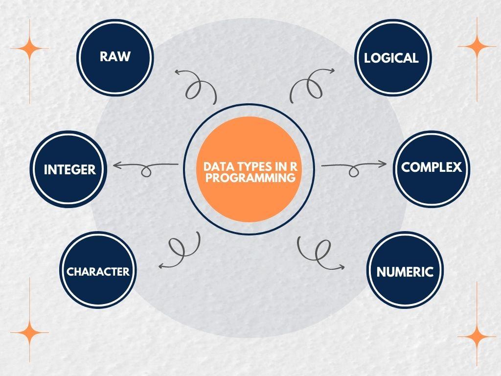

R categorizes data types into atomic (basic, single-element types) and composite (collections of elements). Unlike some languages (e.g., Python, C), R is dynamically typed, meaning you don’t explicitly declare a variable’s type; R infers it at runtime.

Atomic Data Types

• Numeric: Numbers, including integers and decimals.
• Character: Text or strings.
• Logical: Boolean values (TRUE or FALSE).
• Integer: Whole numbers (explicitly defined with L).
• Complex: Complex numbers (e.g., 3 + 2i).
• Raw: Raw bytes (rarely used, e.g., for binary data).

Composite Data Types

• Vector: An ordered collection of elements of the same atomic type.
• List: An ordered collection of elements of different types.
• Matrix: A two-dimensional array of elements of the same type.
• Array: A multi-dimensional collection of elements of the same type.
• Data Frame: A table-like structure with columns of different types.
• Factor: Categorical data for statistical analysis.

2. Detailed Explanation of Data Types

Atomic Data Types

Numeric

Represents numbers, including integers and floating-point decimals.

• Example:

  x <- 42.5  # Floating-point
  y <- 10    # Treated as numeric unless specified as integer
  print(x + y)  # Output: 52.5
  

• Use: Calculations, data analysis (e.g., averages, regressions).

Integer

Explicit whole numbers, denoted with L.

• Example:

  z <- 5L
  print(class(z))  # Output: "integer"
  print(z * 2)     # Output: 10
  

• Use: When integer precision is needed (e.g., indexing, counters).

Character

Text or strings, enclosed in single (') or double (") quotes.

• Example:

  name <- "Alice"
  greeting <- 'Hello, World!'
  print(paste(name, greeting))  # Output: Alice Hello, World!
  

• Use: Storing names, labels, or text data for NLP.

Logical

Boolean values: TRUE (or T) and FALSE (or F).

• Example:

  is_student <- TRUE
  is_teacher <- FALSE
  print(is_student & is_teacher)  # Output: FALSE
  

• Use: Conditional statements, filtering data.

Complex

Numbers with real and imaginary parts (less common).

• Example:

  c <- 3 + 2i
  print(c * 2)  # Output: 6+4i
  

• Use: Scientific computations, signal processing.

Raw

Stores raw bytes (rarely used in typical R programming).

• Example:

  r <- charToRaw("A")
  print(r)  # Output: 41
  

• Use: Low-level data manipulation, binary file handling.

Composite Data Types

Vector

A sequence of elements of the same atomic type, created with c() (combine).

• Example:

  numbers <- c(1, 2, 3, 4)
  names <- c("Alice", "Bob", "Charlie")
  print(numbers * 2)  # Output: 2 4 6 8
  print(names[2])     # Output: "Bob"
  

• Use: Storing lists of values (e.g., ages, scores).
• Note: Vectors are atomic; mixing types (e.g., c(1, "two")) coerces all elements to one kind (here, character).

List

A flexible collection of elements that can have different types, created with list().

• Example:

  mixed_list <- list(42, "Alice", TRUE, c(1, 2, 3))
  print(mixed_list[[2]])  # Output: "Alice"
  print(mixed_list)       # Output: [[1]] 42  [[2]] "Alice"  [[3]] TRUE  [[4]] 1 2 3
  

• Use: Storing heterogeneous data (e.g., a record with name, age, scores).
• Note: Access elements  [[ ]] for single items or [ ] sublists.

Matrix

A two-dimensional array of elements of the same type, created with matrix().

• Example:

  m <- matrix(c(1, 2, 3, 4), nrow=2, ncol=2)
  print(m)
  # Output:
  #      [,1] [,2]
  # [1,]    1    3
  # [2,]    2    4
  print(m %*% m)  # Matrix multiplication
  

• Use: Linear algebra, image processing.

Array

A multi-dimensional collection of elements of the same type, created with array().

• Example:

  arr <- array(1:8, dim=c(2, 2, 2))
  print(arr)
  # Output: 3D array with values 1 to 8
  

• Use: Multi-dimensional data (e.g., 3D image data).

Data Frame

A table-like structure where columns can have different types, created with data.frame().

• Example:

  df <- data.frame(
    name = c("Alice", "Bob"),
    age = c(25, 30),
    is_student = c(TRUE, FALSE)
  )
  print(df)
  # Output:
  #    name age is_student
  # 1 Alice  25       TRUE
  # 2   Bob  30      FALSE
  print(df$age)  # Output: 25 30
  

• Use: Data analysis, storing tabular data (e.g., datasets in CSV files).

Factor

It represents categorical data and is used for statistical modeling.

• Example:

  grades <- factor(c("A", "B", "A", "C"), levels=c("A", "B", "C", "D"))
  print(grades)
  # Output: A B A C
  # Levels: A B C D
  print(summary(grades))
  # Output:
  # A B C D 
  # 2 1 1 0 
  

• Use: Encoding categories (e.g., survey responses, class labels).

3. Type Checking and Conversion

R provides functions to inspect and convert data types:

• Check Type:
  • class()Returns the type or class (e.g., "numeric", "data.frame").
  • typeof()Returns the internal type (e.g., "double", "list").
  • is.<type>()Tests for a specific type (e.g., is.numeric(), is.character()).
• Convert Type:
  • as.<type>()Converts to a specific type (e.g., as.character(), as.numeric()).

Example

x <- 42.5
print(class(x))          # Output: "numeric"
print(is.numeric(x))     # Output: TRUE
y <- as.character(x)
print(y)                 # Output: "42.5"
print(class(y))          # Output: "character"

Note: Coercion may lead to data loss (e.g., as.integer(42.5) yields 42) or NA If conversion fails (e.g., as.numeric("abc")).

4. Practical Example: Combining Data Types

Let’s create a small dataset to demonstrate multiple data types in a data analysis task.

# Create a data frame with student data
students <- data.frame(
  name = c("Alice", "Bob", "Charlie"),
  age = c(20L, 22L, 21L),  # Integer
  score = c(85.5, 90.0, 78.5),  # Numeric
  passed = c(TRUE, TRUE, FALSE)  # Logical
)

# Add a factor for grades
students$grade <- factor(c("A", "A", "B"), levels=c("A", "B", "C"))

# Analyze data
print(students)
# Output:
#      name age score passed grade
# 1   Alice  20  85.5   TRUE     A
# 2     Bob  22  90.0   TRUE     A
# 3 Charlie  21  78.5  FALSE     B

# Calculate average score
avg_score <- mean(students$score)
print(paste("Average Score:", avg_score))  # Output: Average Score: 84.6666666666667

# Filter passing students
passing <- students[students$passed, ]
print(passing)
# Output:
#    name age score passed grade
# 1 Alice  20  85.5   TRUE     A
# 2   Bob  22  90.0   TRUE     A

Explanation:

• Data Types Used: Character (name), integer (age), numeric (score), logical (passed), factor (grade), data frame (students).
• Operations: Creating a data frame, computing averages, and filtering rows.
• Use Case: Represents a typical R workflow for data analysis.

5. Best Practices

• Choose Appropriate Types:
  • Use integer for counts, numeric for decimals, factor for categories.
  • Prefer data frames for tabular data over matrices unless all elements are the same type.
• Check Types:
  • Use class() or str() to verify data types before operations, especially with imported data.
  • Example: str(students) Shows the structure and types of a data frame.
• Handle Coercion Carefully:
  • Be aware of automatic coercion in vectors (e.g., c(1, "2") becomes a character.
  • Validate conversions to avoid NA values.
• Optimize Memory:
  • Use factors for categorical data to save memory.
  • Avoid lists for extensive, uniform data; use vectors or matrices instead.
• Document Code:
  • Comment code to clarify data types, especially in complex analyses.

6. Modern Trends (2025)

• Tidyverse Integration: Packages like dplyr and tibble Enhance data frame manipulation, maintaining type consistency.
• Big Data Support: Libraries like arrow handle large datasets efficiently, preserving R’s type system.
• Interoperability: R integrates with Python (via reticulate) and SQL, requiring careful type mapping.
• Visualization: ggplot2 Leverages factors and data frames for advanced plotting.

7. Next Steps

• Practice: Create a data frame with mixed types and perform analyses (e.g., filter, summarize).
• Learn: Explore free courses (e.g., DataCamp’s Introduction to R, Coursera’s R Programming).
• Experiment: Import a CSV file with read.csv() and inspect its types with str().
• Contribute: Join open-source R projects on GitHub (e.g., tidyverse, data.table).
• Stay Updated: Follow R-bloggers or X posts from R community leaders.

8. Conclusion

R’s data types—atomic (numeric, character, logical, etc.) and composite (vector, list, data frame, etc.)—form the foundation of its data analysis capabilities.
You can efficiently handle statistical tasks by understanding and manipulating these types, from simple calculations to complex modeling. Start with the provided examples, experiment with your datasets, and leverage R’s ecosystem to unlock powerful data insights.