blog posts

Introduction

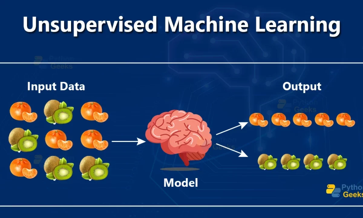
Unsupervised learning is a branch of machine learning where algorithms analyze unlabeled data to uncover hidden patterns, structures, or anomalies without explicit guidance.
Unlike supervised learning, which uses labeled data to predict outcomes, unsupervised learning explores data to find natural groupings or simplified representations. Applications include customer segmentation, data compression, and fraud detection.

This guide explains unsupervised learning concepts, key algorithms, and how to implement them in Python, such as scikit-learn. Practical examples teach you to apply clustering, dimensionality reduction, and anomaly detection, equipping you to tackle real-world problems.

1. What is Unsupervised Learning?

Unsupervised learning involves training models on data without predefined labels or targets. The goal is to infer the underlying structure or relationships within the data.
Consider sorting a pile of mixed fruits into groups based on similarities (e.g., size, color) without knowing the fruit names beforehand.

Key Tasks

• Clustering: Grouping similar data points (e.g., segmenting customers by purchasing behavior).
• Dimensionality Reduction: Simplifying high-dimensional data while preserving structure (e.g., compressing images).
• Anomaly Detection: Identifying unusual or rare data points (e.g., detecting fraudulent transactions).

When to Use Unsupervised Learning

• When labels are unavailable or expensive to obtain.
• To explore data for insights or preprocessing before supervised learning.
• To handle high-dimensional or noisy datasets.

2. Key Unsupervised Learning Algorithms

Clustering

Clustering algorithms group data points based on similarity.

• K-Means: Partitions data into K clusters by minimizing variance within clusters.
• DBSCAN (Density-Based Spatial Clustering of Applications with Noise): Groups points in dense regions, marking outliers as noise.
• Hierarchical Clustering: Builds a tree of clusters, useful for nested groupings.

Dimensionality Reduction

These methods reduce the number of features while retaining essential information.

• Principal Component Analysis (PCA): Using linear transformations, projects data onto a lower-dimensional space.
• t-SNE (t-Distributed Stochastic Neighbor Embedding): Visualizes high-dimensional data in 2D or 3D, emphasizing local structure.
• UMAP (Uniform Manifold Approximation and Projection): Modern alternative to t-SNE, faster and scalable.

Anomaly Detection

Identifies outliers or rare events.

• Isolation Forest: Isolates anomalies using random splits, which is efficient for large datasets.
• One-Class SVM: Learns a boundary around normal data, flagging points outside as anomalies.

3. Python Tools for Unsupervised Learning

Python’s ecosystem is ideal for unsupervised learning. Key libraries include:

• scikit-learn: Core library for clustering, dimensionality reduction, and anomaly detection.
• NumPy: Handles numerical operations and arrays.
• Pandas: Manages data manipulation and analysis.
• Matplotlib/Seaborn: Visualizes results (e.g., cluster scatter plots).
• UMAP-learn: Implements UMAP for dimensionality reduction.
• hdbscan: Advanced density-based clustering.

To install these, run:

pip install scikit-learn numpy pandas matplotlib seaborn umap-learn hdbscan

Jupyter Notebook is recommended for interactive coding and visualization.

4. Practical Examples with Python

Let’s implement three unsupervised learning tasks: clustering, dimensionality reduction, and anomaly detection. These examples use synthetic or standard datasets. For simplicity, they assume you have the required libraries installed.

Example 1: K-Means Clustering

Group customers based on spending and purchase frequency.

import pandas as pd import numpy as np import matplotlib.pyplot as plt from sklearn.cluster import KMeans from sklearn.preprocessing import StandardScaler # Synthetic data data = pd.DataFrame({ 'annual_spend': [500, 2000, 1500, 300, 2500, 800, 2200], 'purchase_frequency': [10, 50, 30, 5, 60, 15, 55] }) # Standardize features scaler = StandardScaler() X_scaled = scaler.fit_transform(data) # Apply K-Means kmeans = KMeans(n_clusters=3, random_state=42) data['cluster'] = kmeans.fit_predict(X_scaled) # Visualize plt.scatter(data['annual_spend'], data['purchase_frequency'], c=data['cluster'], cmap='viridis') plt.xlabel('Annual Spend ($)') plt.ylabel('Purchase Frequency') plt.title('Customer Segmentation with K-Means') plt.show() # Print cluster centers (in original scale) centers = scaler.inverse_transform(kmeans.cluster_centers_) print("Cluster Centers (Spend, Frequency):") for i, center in enumerate(centers): print(f"Cluster {i}: {center}")

Explanation:

• Data: Synthetic customer data with two features.
• Preprocessing: StandardScaler ensures features are on the same scale.
• K-Means: Groups data into 3 clusters based on similarity.
• Visualization: A Scatter plot shows clusters, with colors indicating group membership.
• Output: Cluster centers reveal typical customer profiles (e.g., low spend/low frequency).

Sample Output:

Cluster Centers (Spend, Frequency):
Cluster 0: [ 400.         7.5      ]
Cluster 1: [2100.        55.       ]
Cluster 2: [1500.        30.       ]

Example 2: PCA for Dimensionality Reduction

Reduce the Iris dataset’s dimensions for visualization.

from sklearn.datasets import load_iris from sklearn.decomposition import PCA # Load Iris dataset iris = load_iris() X = iris.data y = iris.target # Used for visualization, not PCA # Standardize features X_scaled = StandardScaler().fit_transform(X) # Apply PCA pca = PCA(n_components=2) # Reduce to 2 dimensions X_pca = pca.fit_transform(X_scaled) # Visualize plt.scatter(X_pca[:, 0], X_pca[:, 1], c=y, cmap='viridis') plt.xlabel('Principal Component 1') plt.ylabel('Principal Component 2') plt.title('Iris Dataset: PCA Reduction to 2D') plt.show() # Explained variance print(f"Explained Variance Ratio: {pca.explained_variance_ratio_}")

Explanation:

• Data: Iris dataset with four features (sepal/petal measurements).
• PCA: Reduces 4D data to 2D, capturing maximum variance.
• Visualization: A Scatter plot shows data points in 2D, colored by accurate labels (for illustration).
• Output: Explained variance ratio indicates how much information is retained.

Sample Output:

Explained Variance Ratio: [0.72962445 0.22850762]

(The first two components capture ~95% of the variance.)

Example 3: Anomaly Detection with Isolation Forest

Detect unusual transactions in a synthetic dataset.

from sklearn.ensemble import IsolationForest # Synthetic transaction data data = pd.DataFrame({ 'amount': [100, 150, 200, 120, 5000, 180, 3000], 'time_of_day': [10, 12, 15, 14, 23, 11, 2] }) # Standardize features X_scaled = StandardScaler().fit_transform(data) # Apply Isolation Forest iso_forest = IsolationForest(contamination=0.3, random_state=42) data['anomaly'] = iso_forest.fit_predict(X_scaled) # Visualize plt.scatter(data['amount'], data['time_of_day'], c=data['anomaly'], cmap='coolwarm') plt.xlabel('Transaction Amount ($)') plt.ylabel('Time of Day (Hour)') plt.title('Anomaly Detection with Isolation Forest') plt.show() # Print anomalies anomalies = data[data['anomaly'] == -1] print("Detected Anomalies:") print(anomalies)

Explanation:

• Data: Synthetic transactions with amount and time features.
• Isolation Forest: Identifies anomalies by isolating points with random splits.
• Parameter: contamination=0.3 Assumes 30% of the data are outliers.
• Visualization: Red points are anomalies, blue are normal.
• Output: Lists transactions flagged as anomalies (e.g., high amounts, unusual times).

Sample Output:

Detected Anomalies: amount time_of_day anomaly 4 5000 23 -1 6 3000 2 -1

5. Data Preprocessing for Unsupervised Learning

Unsupervised learning is sensitive to data quality. Key preprocessing steps:

• Handling Missing Values: Impute with mean/median or remove rows (df.fillna(df.mean())).
• Feature Scaling: Standardize (StandardScaler) or normalize (MinMaxScalerto ensure equal feature influence.
• Outlier Removal: Remove extreme values if they skew results (optional, depends on task).
• Feature Engineering: Create new features (e.g., ratios, aggregations) to enhance patterns.

Example:

# Preprocess data df = pd.DataFrame({'A': [1, np.nan, 3], 'B': [4, 5, 6]}) df.fillna(df.mean(), inplace=True) scaler = StandardScaler() X_scaled = scaler.fit_transform(df)

6. Evaluating Unsupervised Learning Models

Since there are no labels, evaluation relies on intrinsic or task-specific metrics:

• Clustering:
  • Silhouette Score: This score measures how similar points are within clusters compared to between clusters (range: -1 to 1).
  • Inertia: K-Means’ within-cluster variance (lower is better, but not always optimal).
• Dimensionality Reduction:
  • Explained Variance Ratio: PCA’s measure of retained information.
  • Visual Inspection: Check if reduced data preserves meaningful patterns.
• Anomaly Detection:
  • Precision/Recall: If partial labels are available.
  • Domain Expertise: Validate anomalies with business knowledge.

Example (Silhouette Score):

from sklearn.metrics import silhouette_score score = silhouette_score(X_scaled, kmeans.labels_) print(f"Silhouette Score: {score:.2f}")

7. Choosing the Right Algorithm

• K-Means: Best for spherical, well-separated clusters; requires specifying K.
• DBSCAN: Ideal for irregular clusters and outlier detection; no need to set cluster count.
• PCA: Good for linear dimensionality reduction and preprocessing.
• t-SNE/UMAP: Excellent for visualization but computationally intensive.
• Isolation Forest: Efficient for anomaly detection in large datasets.

Tips:

• Use the Elbow Method to choose K in K-Means (plot inertia vs. K).
• Test multiple algorithms and compare results visually or with metrics.
• Consider data size and computational resources (e.g., UMAP is faster than t-SNE).

8. Advanced Topics and Trends (2025)

Advanced Algorithms

• HDBSCAN: Robust density-based clustering, better than DBSCAN for varying densities.
• Autoencoders: Neural networks for non-linear dimensionality reduction (use TensorFlow/PyTorch).
• Gaussian Mixture Models (GMM): Probabilistic clustering for soft assignments.

Example (GMM):

from sklearn.mixture import GaussianMixture
gmm = GaussianMixture(n_components=3, random_state=42)
data['cluster'] = gmm.fit_predict(X_scaled)

Modern Trends

• AutoML for Unsupervised Learning: Tools like H2O.ai automate clustering and anomaly detection.
• Scalable Algorithms: Libraries like RAPIDS (cuML) accelerate clustering on GPUs.
• Explainability: Techniques like SHAP for clustering explain why points are grouped.
• Federated Unsupervised Learning: Analyzes decentralized data while preserving privacy.

9. Challenges and Best Practices

• Challenges:
  • Choosing the correct number of clusters or components.
  • Handling noisy or high-dimensional data.
  • Interpreting results without labels.
• Best Practices:
  • Always scale features before clustering or dimensionality reduction.
  • Visualize results to validate patterns (e.g., scatter plots, heatmaps).
  • Use domain knowledge to interpret clusters or anomalies.
  • Experiment with multiple algorithms and parameters.

10. Next Steps

• Practice: Apply these techniques to Kaggle datasets (e.g., Mall Customer Segmentation, Credit Card Fraud).
• Learn: Explore free courses (e.g., Coursera’s Unsupervised Learning by University of Colorado, Fast.ai).
• Experiment: Try advanced libraries (e.g., HDBSCAN, cuML) or deep learning (autoencoders).
• Contribute: Join open-source projects on GitHub or analyze real-world datasets.

Conclusion

Unsupervised learning in Python unlocks insights from unlabeled data, enabling tasks like customer segmentation, data visualization, and anomaly detection. Mastering algorithms like K-Means, PCA, and Isolation Forest and leveraging libraries like Sci-Kit can help you tackle diverse problems.
Start with the examples provided, experiment with real datasets, and explore advanced techniques to deepen your expertise. With Python’s powerful ecosystem, unsupervised learning is a gateway to discovering hidden patterns in data.