The Excel Date And Time Functions, Date And Time Functions In Excel

Herbert Huffner Excel June 12, 2021

The Excel date and time functions we examine here – including functions

EDATE, YEARFRAC, EOMONTH, NETWORKDAYS.INTL

Four functions are the most widely used in Excel for counting days.

In each of the following functions, we first define that function, then explain the components and how that function works, at which point we must give the function values to perform the calculations for us.

We will then show you an example of a combination of commands in these functions – one of the things you will learn in this step is how to write the formula, which includes steps for function names, parentheses, comma separators, And other components of the command.

Note that arguments are always enclosed in parentheses, and each of these arguments is separated by a comma.

EDATE () function
EDATE is a function to display a date, several months in the past or future, using a record value for future dates and a negative value for past dates. For example, you can use this function to calculate a retirement date or expiration date by calculating an individual’s age from the date of birth or adding a specific number of years to a specific date.

The arguments to this function are:

Start_date: Specify a date to show you the start date (of course, it must be in the correct Excel format in the form of consecutive numbers).
Months: Displays the number of months before or after the start date. And the format of the command is as follows:

= EDATE (start_date, months)

1- For example, here we want to calculate the retirement date for one of our colleagues. You need to open a new worksheet in Excel and in the title field, the names Name, Birthday, Retirement Date, Time Left, and In Years for the column Enter A3, B3, C3, D3, and E3 on this page.
2- In columns A and B, enter the names and dates of birth.
3. Click on cell C4, then go to the Formulas> Data & Time tab and select the EDATE function from the list. You can also enter the formula EDATE () manually in cell C4, ie = EDATE (B4,12 * 62). If you do not want to enter and calculate the number of months, then it is much easier to multiply 12 by the retirement age (ie, 12 months per year multiplied by the age of 62).
4. Copy the formula in cell C4 and paste it in cells C5 to C13, this way you will have the retirement date of each person. Read the next function, the YEARFRAC () function, to see how much time is left for each employee.

YEARFRAC ()

Function This function calculates the number of days between two dates as a decimal number, which will lead to a fraction. This function has special uses because other Excel time and date functions show you only one number.

Use this formula to calculate your retirement date to get an individual age from your date of birth, to be able to calculate the years of these dates, to make sure you get a percentage of the completed year, and the uses There is so much more you can have.

Note that Excel uses whole days between two dates to calculate the fraction of the year as a decimal value.

The arguments used for this function are:

Start_date: (
start date)
End_date: (end-date)
Basis (optional): A type of base for your day (or code)
Then the command to write this is as follows:

= YEARFRAC (start_date, end_date, basis)

Although Excel allows you to put spaces between arguments, you still can not use these spaces between the function and the beginning of parentheses, ie there should be no space between the function and parentheses. Most older timers immediately remove all spaces from their formulas to eliminate the chance of these errors occurring.
Formula

= YEARFRAC (TODAY (), C41)

Enter in cell D4: The start_date argument in this formula is TODAY () – which corresponds to a typical day. The TODAY () function shows you the date today. The date on cell C4 indicates the end date, and the option is based on the number 1, which means the days of the month and the days of the year.
This may seem a bit confusing, but Excel gives you five options for calculating days and years in this formula.

Some accountants in Europe and the United States work on 30-day months and 360-day years; Other systems are based on the days of a month, but still consider a year to be 360 days. And some people define days in months and years arbitrarily.

The codes for each of these modes are written as follows:

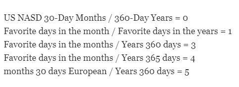When You entered this function, if you hit any key (such as the space key) after the last argument (cell C4), Excel software will open a menu for you that gives you five options in this menu. Select the appropriate code for your work from this list and press Enter.

If you do not enter the base number, the default number will be 0, which means 30 days of the month and 360 days of the year – which you are looking for in real-time. This is the default option for you. not suitable.

The last column (E) in this spreadsheet shows what column D will look like when formatted as a fraction.

For example, E4 cells will be slightly less than 2 years old, while E5 cells are slightly older than 1 year old. E6 cell is equal to 4.1-1 years, cell E7 is equal to 4.8-3 years, and so on.

EOMONTH ()
Function Use this function to specify the date of the last day of the month (future or past). This is because when building a spreadsheet with many calculations, poems and calendars you can not calculate such results using the formulas listed because these formulas give numerical results. This function will show a consecutive number that results in a specific date in Excel.

The arguments to this function are:

Start_date: A date that gives you the start date in a convenient sequential number format in Excel.
Months: This shows you the number of months before or after the start_date.
The coding for this function is = EOMONTH (start_date, months).

For the month’s argument, use positive numbers to indicate the future and negative numbers to indicate the past.

1. Enter ten dates in cells A4 to A13.
2. Enter the formula = EOMONTH (A4,1) in cell B4. Cell A4 is the date for that cell, and the number 1 here means one month. This means that the last day of the month in question is one month past the date in cell A4.

Note that this program will show you a consecutive number in Excel.

3. Then, place your mouse cursor on cell B4 and press the function key F2 (Edit). Do this by moving the cursor over the word A in this formula and pressing the F4 function key three times in a row, or as long as your formula looks like = EOMONTH ($ A4,1).4. For people who are not familiar with this feature, the dollar sign in front of the word A means that the source of the column will not change with the copy of the formula. Now, when we copy this formula to cell A4 and drag it down, the rows of cells will change but the columns will remain the same.
5. Then, set the desired consecutive number in cell B4 in medium-long date format, ie Mon Feb 26, 2016 (meaning Monday, February 26, 2016).
6. Copy cell B4 down from B5 to B13. Note that the medium-long number format will also be copied with the formula.
7. Then, copy this formula in B4 to C4, D4, and E4. Edit each formula to show the new month numbers: Change the number 1 in cell C4 to 6. Change the number 1 in cell D4 to 12 and the number 1 in cell E4 to 18. Now copy cells C4 to E4 into cells C13 to E13.
8. Remember to make the columns wide enough to accommodate new formats, then you will see how quickly you can find this information using this very useful function.

NETWORKDAYS.INTL ()

Function This function calculates the number of business days between two specified dates, other than weekends. This function is useful if you want to calculate the number of working days (or school days) in a year, three months of a year, or a semester.

The difference between this function and other functions is that this function has options by which days can be counted as weekend days. It is not the case for everyone to be closed on Saturdays and Sundays. Some are closed on Mondays and Tuesdays, others are closed on Wednesdays and Fridays. With this function, you can define these weekends for Excel to suit your personal schedule.

In addition, this function allows you to select and set your own rotation days in a specific time format.

For example, in the last quarter of the year of your annual calendar, there are two holidays in October, two holidays in November, and two holidays in December, of course, if you have Halloween and Christmas Eve.

Also, take into account. If you do not take into account these two special nights, then you can set the number of fourth-month holidays from the last three months of the year to six.

The following commands are the codes by which you can define your weekend days to your liking:

Number of weekend days
1. Saturday, Sunday
2. Sunday, Monday
3. Monday, Tuesday
4. Tuesday, Wednesday
5. Wednesday, Thursday overnight
6. Thursday, Friday
7. Friday, Saturday
11. Only Sunday
12. ٫ Only Monday
13. ٫ Only Tuesday
14. ٫ Only Wednesday
15. ٫ Only Thursday
16. ٫ Only Friday
17. ٫ Only Saturday

If you leave this parameter blank (or undefined) in the order, as before Excel assumes it to be 1, meaning it counts your weekends like Saturdays and Sundays.
Enter the holidays as a range of cells, where you specify the main closing dates (such as cells F4 to F10) or a list of consecutive numbers that represent your actual closing dates.

The argument for this function is as follows:

Start_Date: Start Date
End_date: Date
Weekend: Set what days of the week to consider as weekends (additional parameter).
Holidays: A source that indicates that dates should be considered as days when the person is unemployed (additional parameter).
Coding related to the use of this function as

= NETWORKDAYS.INTL (start_date, end_date, [weekend], [holidays])

Is written.
1- On your spreadsheet, start Start Date, End Date, Number of Word Days in the tabs of columns A, B, C, F, and Enter G. Finally, enter the title Holidays (which, as shown above, is placed at the top of both columns F and G in a merged or merged cell.)
2. Enter some random dates in columns A and B. Make sure the End Date column is not pre-dated.
3. Enter the number of random holidays (names and dates) in columns F and G.
4- Place your mouse cursor on cell C4 and go to the Formula tab of Excel and open the Data & Time option and select the NETWORKDAYS.INTL function from this menu.
5. In the Function Arguments dialog box, click inside the Start_Date field box, then click A4.
6. Hold down the Tab key on the End_Date field box and use your mouse to click on cell A4.
7. Hold down the Tab key on the Weekend field and enter one of the defined weekend codes in it (remember that the number 1 means Saturday and Sunday).
8. Press and hold the Tab key on the Holidays field, then select or highlight cells G4 to G11, and then click OK.
Before copying this formula from cell C4 into cells C5 through C11, use the function key F4 to positive the Holiday cells: Command