Training data types in programming with R
Generally, when programming in any language; You have to use different variables to be able to store different information. Variables alone: They are nothing but occupy parts of memory to store values in them.
This means that when you create a variable, you take up space in the memory of the device.
You may want information about different types of data such as characters, integers; Decimal audit numbers; Store decimal numbers, boolean variables, and more. Based on the variable data types, the operating system allocates memory and decides what can be stored in the stored memory.
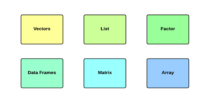
Unlike other programming languages such as C and Java; In R, variables are not defined as a type of data. Variables are assigned to R objects, and R-object data types are converted to variable data types. There are many types of R objects. Frequently used ones are:
- Vectors
- Lists
- matrix
- Arrays
- Facts
- Data frameworks
The simplest of these objects; It is an object vector and there are six types of data from these tiny vectors, also known as six classes of vectors.
Other R objects are built on vectors.
| data type | Example | Becoming |
| Logical | TRUE (correct); FALSE |
The output of this code is as follows:
|
| Numerical | 12.3, 5, 999 |
The output of this code is as follows:
|
| Integer | 2L, 34L, 0L |
The output of this code is as follows:
|
| mixed | 3 + 2i |
The output of this code is as follows:
|
| character | “A”, “good”, “TTUE”, “23.4” |
The output of the above code is as follows:
|
| Raw | “Hello” in the form 48 65 6c 6c 6f Is saved. |
The above output is as follows:
|
In R programming, very basic data types; Objects are R- and are called vectors , as shown above; Holds elements of different classes. Please note that the number of classes in R is not limited to the above six types.
For example, we can use many vectors to create an array whose class becomes an array.
Vectors
When you want to create vectors with more than one element; You can use the function () c, which means to combine elements into one vector.
# Create a vector.
apple <- c (‘red’, ‘green’, ”yellow”)
print (apple)
# Get the class of the vector.
print (class (apple))
When we run the above code; The following results are generated:
[1] “red” “green” “yellow”
[1] “character”
Lists
A list is actually an R object that contains different types of elements within itself. In fact, the elements in the list can include vectors, functions, and even another list.
# Create a list.
list1 <- list (c (2,5,3), 21.3, sin)
# Print the list.
print (list1)
When we run the above code; The following result is obtained:
[[1]]
[1] 2 5 3
[[2]]
[1] 21.3
[[3]]
function (x) .Pimitive (“sin”)
matrix
one matrix; It is actually a rectangular data set. The matrix can be created using a vector that is used as input to the matrix function.
# Create a matrix.
M = matrix (c (‘a’, ‘a’, ‘b’, ‘c’, ‘b’, ‘a’), nrow = 2, ncol = 3, byrow = TRUE)
print (M)
When we run the above code; The following result is obtained:
[, 1] [, 2] [, 3]
[1,] “a” “a” “b”
[2,] “c” “b” “a”
Arrays
While matrices are limited to two dimensions; Arrays can have any number of dimensions. The array function has a property that can be used to create any number of dimensions for arrays. In the following example, we create an array with two elements that are matrices.
# Create an array.
a <- array (c (‘green’, ‘yellow’), dim = c (3,3,2))
print (a)
When we run the above code; The following result is obtained:
,, ۱
[, 1] [, 2] [, 3]
[1,] “green” “yellow” “green”
[2,] “yellow” “green” “yellow”
[3,] “green” “yellow” “green”
,, ۲
[, 1] [, 2] [, 3]
[1,] “yellow” “green” “yellow”
[2,] “green” “yellow” “green”
[3,] “yellow” “green” “yellow”
Factors
Factors are r-objects that are created using a vector in which the distinct values of the elements in the vector are labeled. These labels are always characters, regardless of whether the inputs of the vectors are numerical or character or boolean variables.
Invoices are created using the factor () function . The nlevels function gives us the number of levels.
# Create a vector.
apple_colors <- c (‘green’, ‘green’, ‘yellow’, ‘red’, ‘red’, ‘red’, ‘green’)
# Create a factor object.
factor_apple <- factor (apple_colors)
# Print the factor.
print (factor_apple)
print (nlevels (factor_apple))
When we execute the above code; The following result is obtained:
[1] green green yellow red red red green
Levels: green red yellow
[1] 3
Data frameworks
Data frameworks are tabular data objects. Unlike matrices, in a data framework; Each column can contain different modes of data. The first column can have numeric values; While the second column can be a character; The third column can also be logical. This is a list of vectors of equal length.
Data frames are created using the data.frame () function .
# Create the data frame.
BMI <- data.frame (
gender = c (“Male”, “Male”, “Female”),
height = c (152, 171.5, 165),
weight = c (81.93, 78),
Age = c (42,38,26)
)
print (BMI)
When we run the above code; The following results are generated:
gender height weight Age
1 Male 152.0 81 42
2 Male 171.5 93 38
3 Female 165.0 78 26