R and RStudio programming training in 40 minutes! (For beginners)
R is a free and open source programming language developed in 1995 at the University of Auckland as an environment for statistical and graphical computing.
In this article, in the form of a few pages published by the university itself, you will learn R&R Studio in simple language. Bookmark this page in your browser. With this extremely concise yet complete article, you will not need another source.
1- General plan
1- Overview of education
- Review training goals
- Why is this training necessary?
2- What is R?
- Why should I use R?
- R What can it do?
3- How to start?
- RStudio interface
- How to import, export and view files
- How to navigate the Help tab
- What is a package?
- How to save files
2- Overview of education
1-2 Training goals
- Develop solutions to investigate soil correlation problems and update activities
- Evaluate reviews for interpretive results and determine how they work
- Create a continuous level of point data
- Data collection for the population at NASIS
2-2 Why is this training necessary?
- Opportunities to learn these techniques are limited, especially at the undergraduate level
- Compatible method (data analysis, data population, sampling design, etc.)
- There is a constant need to use these methods more:
- Mapping of lands with high production rates
- Ecological sites
- Soil treatment (separation)
3- What is R?
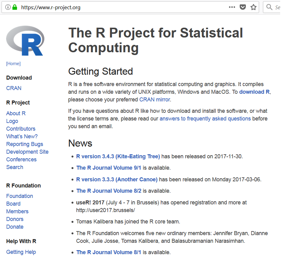
R is a free and open source programming language developed in 1995 at the University of Auckland as an environment for statistical and graphical computing. Since then, R has become one of the dominant software environments for data analysis and is used by various disciplines including soil science, environment and geoinformatics. It is especially popular because of its graphical capabilities, but it is very popular because of its GIS capabilities, which make it relatively easy to produce raster-based models. Recently, R has also acquired various packages specifically designed for the analysis of soil data.
1- Software environment:
- statistics
- Graphics
- Programming
- calculator
- GIS
- Etc…
2- Language for exploring, summarizing and modeling data
- Functions = Verbs
- Objects = noun
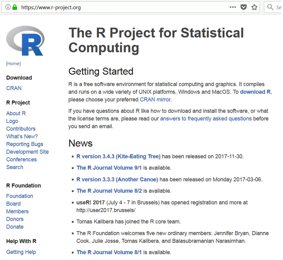
1-3 Why should we learn R?
While the vast majority of people use Excel to analyze data, R has numerous benefits, including:
1- The cost of using R is free!
2- Repeatable research (documentation, repetition)
- Repeat:
- Code + output in a document
- Next time easier
- There are many excel horror stories from misguided scientific studies (TED talk)
- Scalability: Can be used for small or large issues
3- R in forums
- R User Groups (including R-Ladies)
- Stack Overflow
4- Learning resources (quantitative and qualitative)
- R books
- (Free Online) R Books
5. R is becoming the new norm. “If we do not accept these challenges, other less qualified people will accept the challenge.”
While some people find the use of the command line environment daunting, as the volume and variety of data increases, this is a necessary skill for scientists. Therefore, programming or scripting, in addition to their native language and their specific terms, has become a third language for many scientists. Other popular programming languages include SQL (eg NASIS), Python (eg ArcGIS and JavaScript)
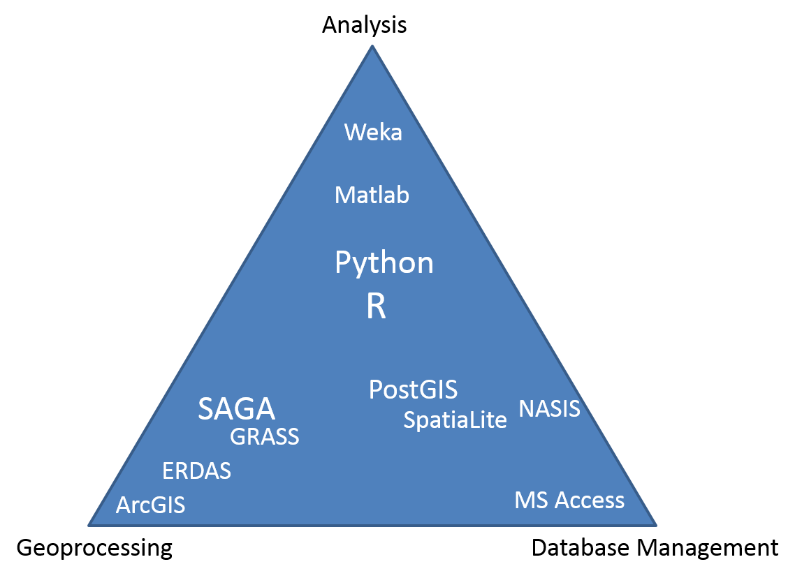
2-3 What can R do?
1-2 packages
- Base R (performance extends through packages)
- Basic summaries of quantitative or qualitative data
- Data exploration through graphics
- Processing and analysis of GIS data
- R Soil Science Packages
- aqp – illustration, aggregation, classification
- groundDB – Access to commonly used soil databases
- axaReports – A handful of reporting templates
- soiltexture – texture triangles
- Environmental R packages
- vegan – grammar, diversity analysis, etc.…
- dismo – Species distribution model
2-3-2 Soil science applications
1-2-2 2-3 Creating maps
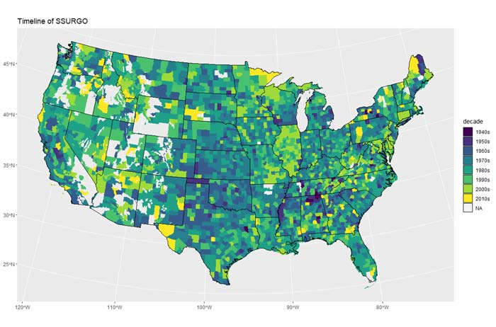
2-2-2-3 Drawing soil profiles
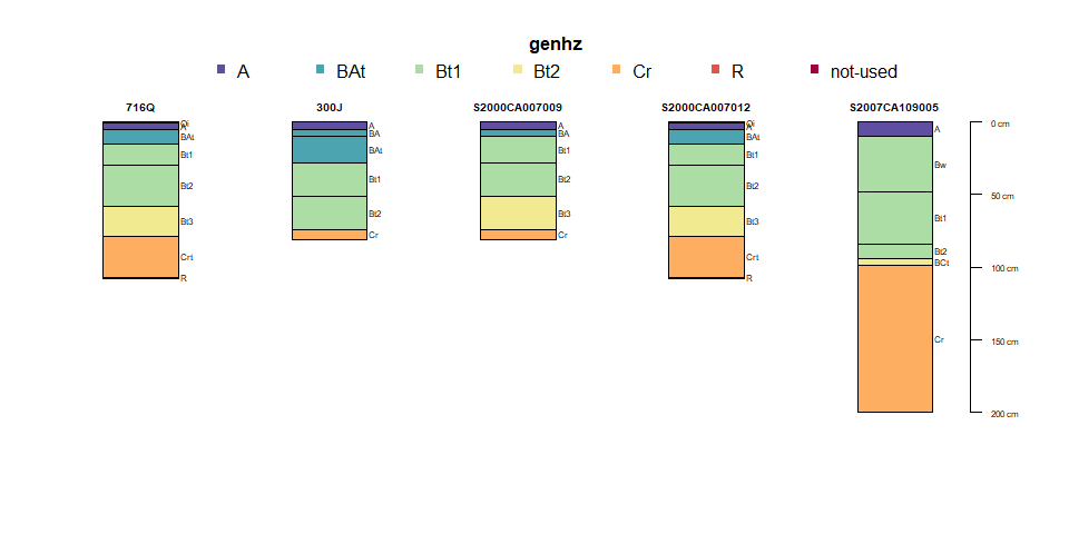
3-2-2-3 Draw depth charts
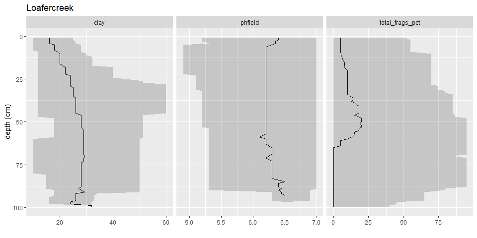
4-2-2-3 Specification Range Estimation (RIC)
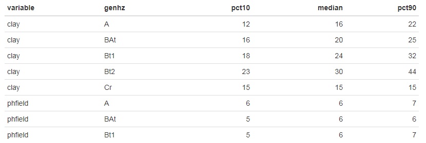
RStudio: An integrated development environment (IDE) for R.
RStudio is an integrated development environment (IDE) that lets you interact with R more easily. RStudio is similar to the standard RGui, but more user-friendly. It has drop-down menus, multi-leaf windows and more personalization options. The first time you open RStudio, you will see three windows. The fourth window is hidden by default, but opens the File drop-down menu, then New File and then R Script.
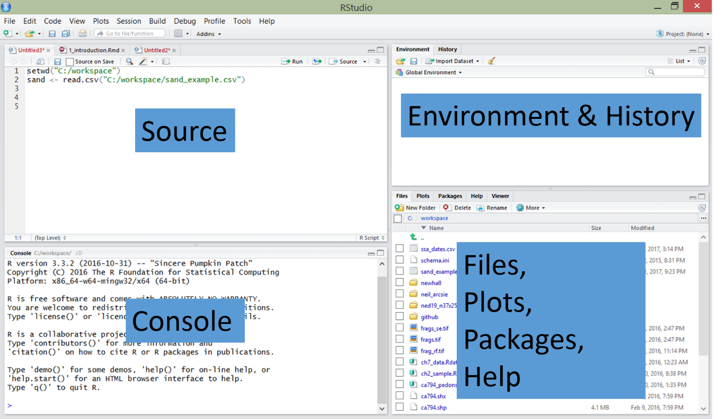
| Window / Header R Studio | Place | Description |
| Console window | Bottom left | Where input commands are entered and output output |
| Source tabs | Top left | Internal text editor |
| Environment tab | Top right | Interactive list of loaded R objects |
| History tab | Top right | List of keys entered into the console |
| Files tab | Bottom right | Explorer file for navigating C drive folders |
| Plots tab | Bottom right | Output location for charts |
| Tab Packages | Bottom right | List of installed packages |
| Help tab | Bottom right | Output locations for help commands and help search window |
| Viewer tab | Bottom right | Advanced tab for local web content |
1-4 USDA computer setup
R and RStudio are installed on all USDA computers that have NASIS installed. R and RStudio are usually updated once a year and are CCE approved. Versions available on USDA devices may be available for public download one to three before the latest version. Having an outdated version of R rarely causes a problem, although it may give some warnings.
2-4 Basic points for using R
You need to type or copy and paste the commands after the command line (>) that appears when R is opened. After typing the command in console R and pressing Enter on the keyboard, this command is executed. If the command is incomplete, R continues the declaration (indicated by a plus sign: +). You can also write a script in the script window and select a command and click the Run button.
R is case sensitive. Make sure the spelling and capitalization of the letters are correct.
The commands in R are also called functions. The basic format of a function in R is:
object <- function.name (argument_1 = data, argument_2 = TRUE)
The up arrow (^) on the keyboard can show you the previous commands you typed in console R.
The $ symbol is used to select a specific column in a table (for example, table $ column).
You must use the # symbol before any text you do not want R to run (such as comments, notes, or instructions). R ignores the rest of the script line below #.
for example:
plot (x, y) # This text will not affect the plot function because of the comment
1- 2-4 Brief example
# Addition
1 + 1
[1] ۲
# Multiplication
10 * 10
[1] 100
# Compute Logarithm
log10 (100)
[1] ۲
# Print Text
Hello World
[1] “Hello World”
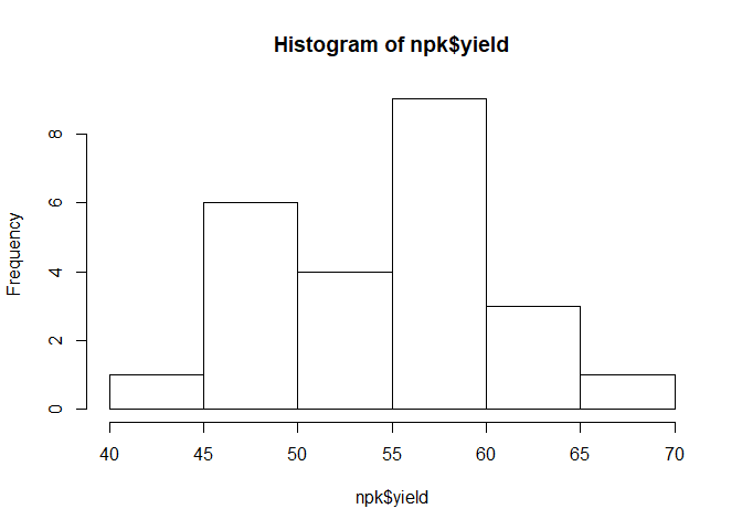
# Plot Histogram
hist (npk $ yield)
# Assignment
test <- 1
# or
test = 1
3-4 work directories
1-3-4 Setting a business directory
Before you start working on R, you need to set up your work directory (a folder to hold all your project files). for example
“C: \ workspace2 \…”.
To change the directory in RStudio, select the main menu Session >> Set Working Directory >> select. Or from the “Files” tab, click More >> Set As Working Directory to use the current location of the “Files” tab as your work directory.
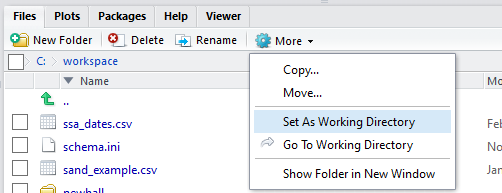
Setting up a work directory through menus is the same thing as setting up a console with the setwd () command:
setwd (“C: / workspace2”)
This directory is where all your input data should be stored and is also the default location for chart files and other output.
Basically you want to find your code entries in the job directory so you can access them using file paths. File paths will be easier if you move the folder containing your script (s) around.
Note: Be careful when specifying file paths R uses slash / instead of back slash \.
To check the path to the current directory file (which should now be “C: \ workspace2”), type:
getwd ()
2-3 3-4 RStudio projects (.Rproj files)
You can also manage your work directory using RStudio Projects. A project file (RStudio.
You can open or create projects using the drop-down menu in the upper right corner of the RStudio window (shown below)
![]()
See the regular Project drop-down menu here:
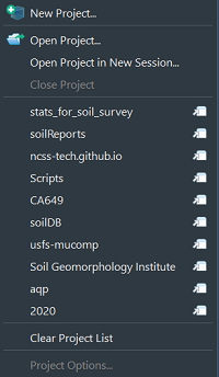
Using “New Project…” you can create new projects from existing or new directories.
When you click “Open Project”, your work directory is automatically set to the location of the .Rproj file – which is very useful.
Any recently created or used project will be displayed in the “Project List”.
Keeping project-specific business directories simple is just a good way to help you keep code and input data organized and get back to it after a while away from the project.
4-4 Data management in RStudio
1-4-4 Enter data
After setting up your work directory, you can import data from csv, .txt and so on. A basic command for importing data into R () is read.csv. This command is followed by the file name and then some optional instructions on how to read the file.
First, create a sample file by copying the content below. Paste the content into Notepad and save the file as sand_example.csv in your C: \ workspace2 folder.
location, landuse, horizon, depth, sand
city, crop, A, 14,19
city, crop, B, 25,21
city, pasture, A, 10,23
city, pasture, B, 27,34
city, range, A, 15,22
city, range, B, 23,23
farm, crop, A, 12.31
farm, crop, B, 31,35
farm, pasture, A, 17.30
farm, pasture, B, 26.36
farm, range, A, 15.25
farm, range, B, 24.29
west, crop, A, 13,27
west, crop, B, 29.25
west, pasture, A, 11,21
west, pasture, B, 31.26
west, range, A, 14.23
west, range, B, 24,24
This dataset can be entered into R using the Import Dataset button from the Environment tab or by typing the following command in console R:
sand <- read.csv (“C: /workspace2/sand_example.csv”)
# if your workspace was already set you could simply use the filename, like so
sand <- read.csv (“sand_example.csv”)
1- 1-4-4 Notes on Microsoft Excel files
R can import Excel files, but generally using Excel is a bad idea. Excel has a dangerous default that automatically converts data to its standard format with common symbols without warning. For example, the “11-JUN” character enters an automated cell on 11/6/2017, even if the data is still displayed as 11-JUN. The only way to prevent this default behavior is to manually enter your data into Excel via Data Tab> Get External Data Ribbon and manually adjust the data type of all columns on the text.
2-4-4 Exporting data
Use the write.csv () command to export data from R. Because we have configured our work directory, R saves our file automatically in the work directory.
write.csv (sand, file = “sand_example2.csv”)
# or use the write.table () function to export other text file types
3-4-4 View and delete data
After importing the file, you need to check that R has entered your information correctly. Make sure the numeric data is entered correctly, your column headings are saved, and so on. To view the data, just click on the sand data set listed in the Environment tab, which will open a separate tab that shows a spreadsheet like the one below.
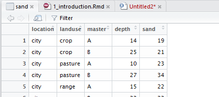
In addition, you can use the following functions to view your data in R.
| Function | Description |
| Print () | Prints the whole object (avoid large tables) |
| Head () | The first 6 lines print your data |
| Str () | Shows the data structure of an R object |
| Names () | The column name (for example, title) lists your data |
| Ls () | Lists all R objects in your workspace list |
Enter the following commands to view the sand data set in R:
str (sand)
names (sand)
head (sand)
ls ()
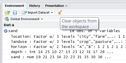
A data object is anything you create or enter and assign a name to in R. The Environment tab lets you see what data objects are in your R session and expand their structure. Currently sand should be the only data object listed. If you want to remove all data objects from your R session, you can click the sweep icon from the Environments tab. Otherwise you can type:
# Remove all R objects
rm (list = ls (all = TRUE))
# Remove individual objects
rm (sand)
5-4 Get help
R has extensive documentation, numerous mailing lists, and countless books (many of which are free). Internal help files are sometimes encrypted and online responses can be minor, but you can find them if you are looking for help. To learn more about the function you use and the options and arguments available, learn to help yourself by using some of the following guide functions in RStudio:
1. Use the Help tab in the lower right window to search for commands (such as hist) or topics (such as histograms).
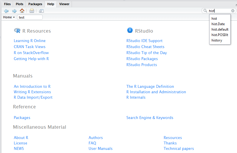
To display the help screen, type help (read.csv or? Read.csv) in the console window. The results will appear in the Help tab in the lower right window. Some functions may need to be quoted, such as ( “+”) Help.
# Help file for a function
help (read.csv) # or? read.csv
# Help files for a package
help (package = “soiltexture”)
1-4-4 Exercise: Check the read.csv () function.
Read the help file for the read.csv () function. How can the first row of the sand data set not be interpreted as a header?
6- 4 packages
Packages are a set of additional functions that can be downloaded. They usually contain sample data that can be used to represent these functions. Although R has many common statistical functions and models, most of our work requires additional packages.
1-4-4 Installing packages
To use a package, you must first install it and then download it. These steps can be done on the command line or using the Packages tab. The following are examples of both methods. R packages are installed only once (until R is upgraded or reinstalled). Each time you start a new R session, you must download the package that you want to use in that session.
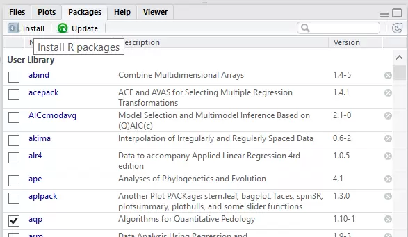
In the Packages tab, you will see a list of all the packages installed on your computer and 2 buttons titled “install” or “update”. To install the new package, just select the Install button. You can enter one or more packages while separating a comma.
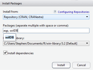
Use the following commands to find out what packages are installed on your computer:
library ()
# or
installed.packages ()
A very useful package for soil scientists is the soiltexture package, which, as you would expect, allows you to draw soil texture triangles. If you have not already downloaded this package, the following command shows how to install it:
# CRAN (static version)
installed.packages (c (“aqp”, “soilDB”, “soilReports”, “soiltexture”))
# GitHub (development version)
devtools :: install_github (“ncss-tech / soilDB”, dependencies = FALSE, upgrade_dependencies = FALSE, build = FALSE)
2-4-4 Loading packages
After installing the package, it must be loaded in session R to be used.
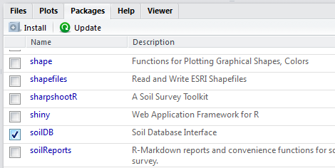
library (soiltexture)
By checking the box next to the package name, you can download packages using the Packages tab. The soiltexture package documentation of the help functions is available in R.
help (package = “soiltexture”)
This help command sends you to a web page. Scroll down and select the “TT.plot” link. This link displays a web page with instructions on how to use the TT.plot () function in R.
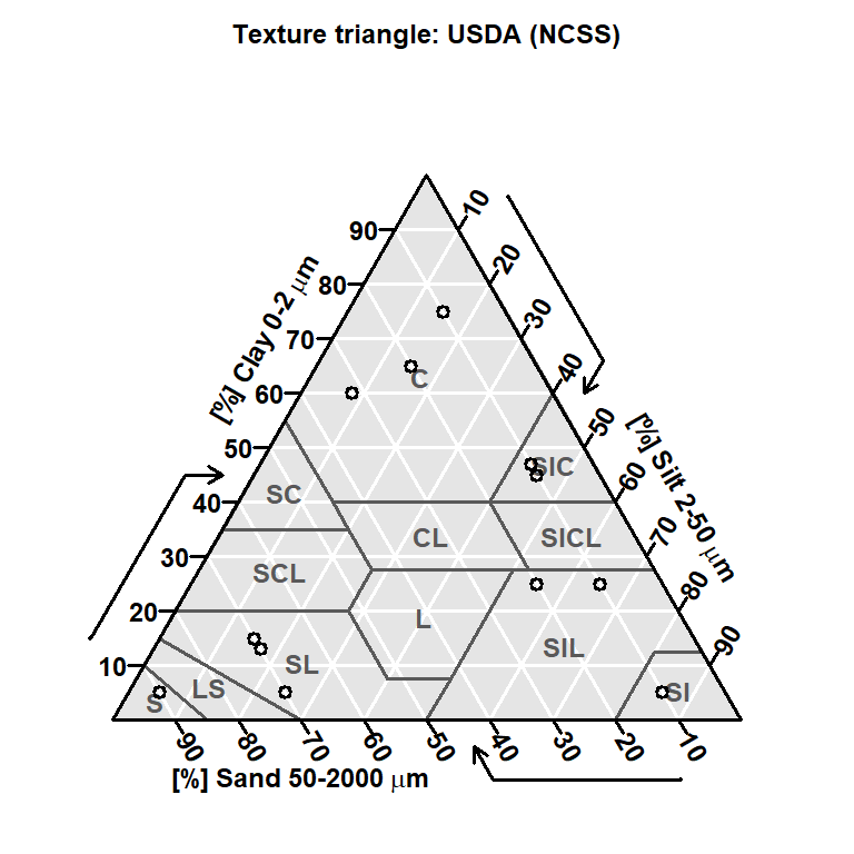
The main application of TT.plot () is the TT.plot (class.sys) function, tri.data. The “class.sym” argument specifies a string of characters that names the text classification system.
# Copied from soiltexture vignette
# Create a dummy data frame of soil textures:
example <- data.frame (
CLAY = c (05,60,15,05,25,05,25,45,65,75,13,47),
SILT = c (05,08,15,25,55,85,65,45,15,15,17,43),
SAND = c (90,32,70,70,20,10,10,10,20,10,70,10),
OC = c (20,14,15,05,12,15,07,21,25,30,05,28)
)
TT.plot (class.sys = “USDA-NCSS.TT”, tri.data = example)
7-4 script writing
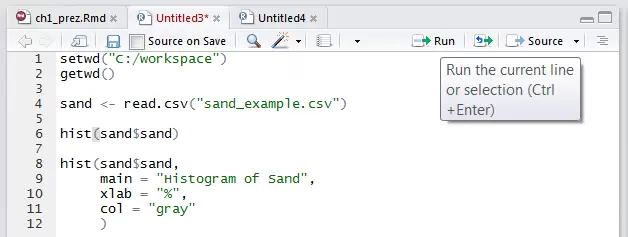
RStudio source tabs work as an internal text editor. Commands are usually written (or scripted) before using the R functions in the console. Scripting is basically showing your work. The sequence of functions needed to complete a task in order to document or automate a scripted task. Although scripting may be cumbersome at first, it can save time in the long run, especially for repetitive tasks. Benefits include:
- Allows others to produce your work, which is the foundation of science
- Acts as instructions / reminders on how to do a task
- Enables fast repetition, which saves time and evaluates gradual changes
- Reduces the likelihood of human error
1-7-4 Basic tips for scripting
To write a script, just open a new R script file by clicking File> New File> R Script. In the text editor, type a sequence of functions.
- Put each function (eg read.csv ()) on a separate line.
- If a function has a long list of arguments, put each argument on a separate line.
- You can delete a command from the text editor by placing the cursor on a line and typing Crtl + Enter, or by clicking the Run button.
- You can delete a complete R script file by clicking the Source button.
8-4 Save R files
In R you can save several types of files to track what you do. File types include: workspace, scripts, history and graphics. It is important to save often because R, like any other software, may crash periodically. Such problems are especially common when working with large files. You can save your workspace in R via the command line or File menu.
1- 8-4 script .R) R)
The R script is simply a text file of the R commands you typed.
You may want to save your scripts (whether written in R Editor or another program such as Notepad) so that you can refer to them in the future, edit them, and keep track of your tasks. To save R scripts in RStudio, just click the save button from the R script tab. Save scripts with a .R extension. R assumes that script files are saved with only that extension. If you use another text editor, you will no longer have to worry about storing your scripts in R. You can open text files in the RStudio text editor, but be careful to copy and paste Word files, as explained below.
Click the file icon to open the R script.
1-1-4-4 Notes on Word files
It is generally a bad idea to use Microsoft Word to write or save R scripts. Some keyboard characters, such as quotes, are not stored uniformly in Word (for example, “vs.”). The difference is largely indistinguishable to the human eye, but will not work in R.
2-8-4 workspace (.Rdata)
The R workspace (or workspace) contains all the data objects that you have created or loaded in your R session. When you turn off R by typing q () or exiting the application window, it asks you to save your workspace. If you select yes, R saves a file named .RData to its work directory. The next time you open R and reload your .Rdata workspace, all your data objects will be available in R, and all the commands you typed can be used using the up and down arrow keys on the keyboard. Are accessible. You can also save or upload your workspace from the menu at any time from your R session by clicking Session> Save Workspace As .. or click the save button on the Environment tab.
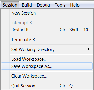
R command to save your workspace:
save.image (file = ”workspace.RData”)
3-8-4 History of R (.Rhistory)
The R history file is a copy of all your keystrokes. Like the R file, the Rhistory file is a text file that lists all the commands you have executed. Does not record a record of results. Click the Open File or Save button to load or save the R history from the History tab. If you download the Rhistory file, your previous commands will be available again with the up and down arrow keys.
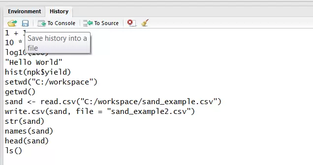
You can also use the command line to load or save your history.
savehistory (file = “sand.Rhistory”)
loadhistory (file = “sand.Rhistory”)
history (max.show = Inf) #displays all previous commands
4-8-4 Graphics R
Graphic outputs can be stored in various formats.
| format | Function |
| pdf (“graphic.pdf”) | |
| Windows metafile | win.metafile (“graphic.wmf”) |
| png | (“Graph.png”) png |
| jpeg | (“Graph.jpg”) bmp |
| bmp | (“Graph.ps”) postscript |
| postscript |
To save the chart: (1) Click on the Plots Tab window 2) Click the Export button, 3) Select the format you want (3) Change the export settings to your liking, and (4) Click Save.
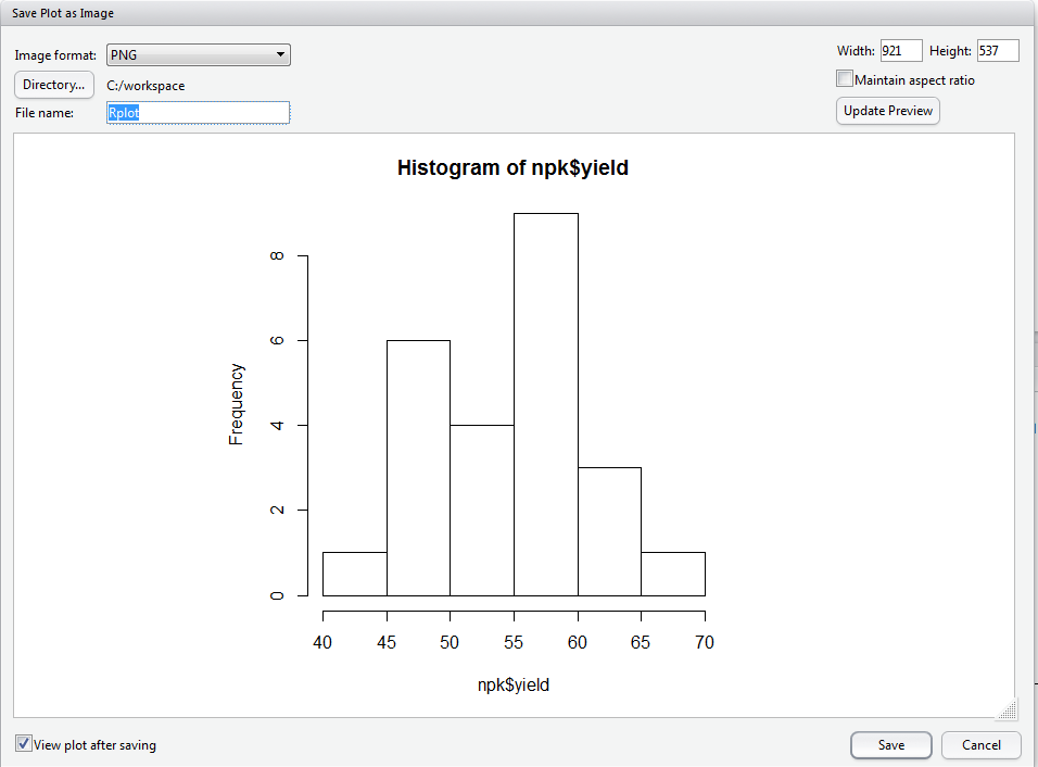
R command to save a chart:
png (file = “npk_yield.png”)
plot (npk $ yield)
dev.off ()
The first line of this command creates a blank file called sand with the JPEG extension. The second line draws the data object from which you want to create a graph (here is the JPEG file that we are creating). The third line closes the graphics device.
5- Rcmdr (Commander R): Graphical user interface for R
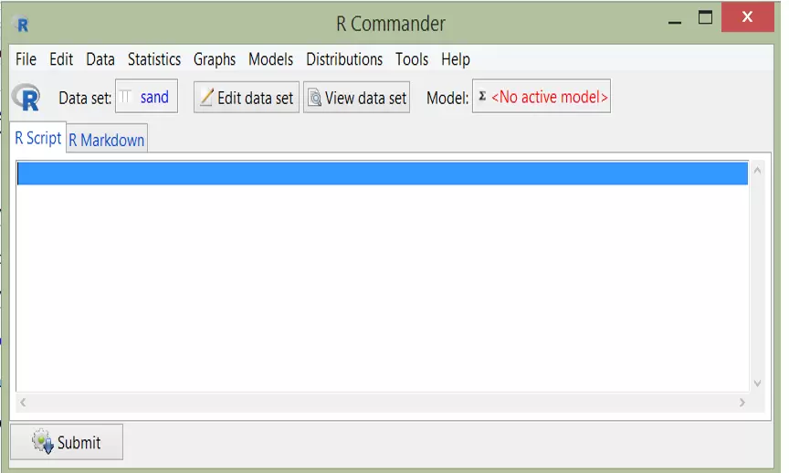
While we recommend using RStudio for some of the above reasons, many newcomers to R can benefit from a graphical user interface (GUI) that allows the user to use basic functions. Run from a point and click interface. Fortunately, R for Beginners has R Commander (Rcmdr) GUI, which is similar to JMP.
Rcmdr was created by John Fox for his elementary statistical students so that they can see how the software works without having to learn a lot of function names and arguments.
Though Rcmdr is a great way to get acquainted with R and statistics in a GUI environment.
The Rcmdr can be opened quickly by entering the following command in console R.
install.packages (Rcmdr)
library (Rcmdr)
In this article, in the form of a few pages published by the university itself, you will learn R&R Studio in simple language. Bookmark this page in your browser. With this extremely concise yet complete article, you will not need another source.
1- General plan
1- Overview of education
- Review training goals
- Why is this training necessary?
2- What is R?
- Why should I use R?
- R What can it do?
3- How to start?
- RStudio interface
- How to import, export and view files
- How to navigate the Help tab
- What is a package?
- How to save files
2- Overview of education
1-2 Training goals
- Develop solutions to investigate soil correlation problems and update activities
- Evaluate reviews for interpretive results and determine how they work
- Create a continuous level of point data
- Data collection for the population at NASIS
2-2 Why is this training necessary?
- Opportunities to learn these techniques are limited, especially at the undergraduate level
- Compatible method (data analysis, data population, sampling design, etc.)
- There is a constant need to use these methods more:
- Mapping of lands with high production rates
- Ecological sites
- Soil treatment (separation)
3- What is R?
R is a free and open source programming language developed in 1995 at the University of Auckland as an environment for statistical and graphical computing. Since then, R has become one of the dominant software environments for data analysis and is used by various disciplines including soil science, environment and geoinformatics. It is especially popular because of its graphical capabilities, but it is very popular because of its GIS capabilities, which make it relatively easy to produce raster-based models. Recently, R has also acquired various packages specifically designed for the analysis of soil data.
1- Software environment:
- statistics
- Graphics
- Programming
- calculator
- GIS
- Etc…
2- Language for exploring, summarizing and modeling data
- Functions = Verbs
- Objects = noun
1-3 Why should we learn R?
While the vast majority of people use Excel to analyze data, R has numerous benefits, including:
1- The cost of using R is free!
2- Repeatable research (documentation, repetition)
- Repeat:
- Code + output in a document
- Next time easier
- There are many excel horror stories from misguided scientific studies (TED talk)
- Scalability: Can be used for small or large issues
3- R in forums
- R User Groups (including R-Ladies)
- Stack Overflow
4- Learning resources (quantitative and qualitative)
- R books
- (Free Online) R Books
5. R is becoming the new norm. “If we do not accept these challenges, other less qualified people will accept the challenge.”
While some people find the use of the command line environment daunting, as the volume and variety of data increases, this is a necessary skill for scientists. Therefore, programming or scripting, in addition to their native language and their specific terms, has become a third language for many scientists. Other popular programming languages include SQL (eg NASIS), Python (eg ArcGIS and JavaScript)

2-3 What can R do?
1-2 packages
- Base R (performance extends through packages)
- Basic summaries of quantitative or qualitative data
- Data exploration through graphics
- Processing and analysis of GIS data
- R Soil Science Packages
- aqp – illustration, aggregation, classification
- groundDB – Access to commonly used soil databases
- axaReports – A handful of reporting templates
- soiltexture – texture triangles
- Environmental R packages
- vegan – grammar, diversity analysis, etc.…
- dismo – Species distribution model
2-3-2 Soil science applications
1-2-2 2-3 Creating maps

2-2-2-3 Drawing soil profiles

3-2-2-3 Draw depth charts

4-2-2-3 Specification Range Estimation (RIC)

RStudio: An integrated development environment (IDE) for R.
RStudio is an integrated development environment (IDE) that lets you interact with R more easily. Then RStudio is similar to the standard RGui, but more user-friendly. It has drop-down menus, multi-leaf windows and more personalization options. The first time you open RStudio, you will see three windows. The fourth window is hidden by default, but opens the File drop-down menu, then New File and then R Script.

| Window / Header R Studio | Place | Description |
| Console window | Bottom left | Where input commands are entered and output output |
| Source tabs | Top left | Internal text editor |
| Environment tab | Top right | Interactive list of loaded R objects |
| History tab | Top right | List of keys entered into the console |
| Files tab | Bottom right | Explorer file for navigating C drive folders |
| Plots tab | Bottom right | Output location for charts |
| Tab Packages | Bottom right | List of installed packages |
| Help tab | Bottom right | Output locations for help commands and help search window |
| Viewer tab | Bottom right | Advanced tab for local web content |
1-4 USDA computer setup
R and RStudio are installed on all USDA computers that have NASIS installed. R and RStudio are usually updated once a year and are CCE approved. Versions available on USDA devices may be available for public download one to three before the latest version. Having an outdated version of R rarely causes a problem, although it may give some warnings.
2-4 Basic points for using R
You need to type or copy and paste the commands after the command line (>) that appears when R is opened. After typing the command in console R and pressing Enter on the keyboard, this command is executed. If the command is incomplete, R continues the declaration (indicated by a plus sign: +). You can also write a script in the script window and select a command and click the Run button.
R is case sensitive. Make sure the spelling and capitalization of the letters are correct.
The commands in R are also called functions. The basic format of a function in R is:
object <- function.name (argument_1 = data, argument_2 = TRUE)
The up arrow (^) on the keyboard can show you the previous commands you typed in console R.
The $ symbol is used to select a specific column in a table (for example, table $ column).
You must use the # symbol before any text you do not want R to run (such as comments, notes, or instructions). R ignores the rest of the script line below #.
for example:
plot (x, y) # This text will not affect the plot function because of the comment
1- 2-4 Brief example
# Addition
1 + 1
[1] ۲
# Multiplication
10 * 10
[1] 100
# Compute Logarithm
log10 (100)
[1] ۲
# Print Text
Hello World
[1] “Hello World”
# Plot Histogram
hist (npk $ yield)

# Assignment
test <- 1
# or
test = 1
3-4 work directories
1-3-4 Setting a business directory
Before you start working on R, you need to set up your work directory (a folder to hold all your project files). for example
“C: \ workspace2 \…”.
To change the directory in RStudio, select the main menu Session >> Set Working Directory >> select. Or from the “Files” tab, click More >> Set As Working Directory to use the current location of the “Files” tab as your work directory.

Setting up a work directory through menus is the same thing as setting up a console with the setwd () command:
setwd (“C: / workspace2”)
This directory is where all your input data should be stored and is also the default location for chart files and other output.
Basically you want to find your code entries in the job directory so you can access them using file paths. File paths will be easier if you move the folder containing your script (s) around.
Note: Be careful when specifying file paths R uses slash / instead of back slash \.
To check the path to the current directory file (which should now be “C: \ workspace2”), type:
getwd ()
2-3 3-4 RStudio projects (.Rproj files)
You can also manage your work directory using RStudio Projects. A project file (RStudio.
You can open or create projects using the drop-down menu in the upper right corner of the RStudio window (shown below)
![]()
See the regular Project drop-down menu here:

Using “New Project…” you can create new projects from existing or new directories.
When you click “Open Project”, your work directory is automatically set to the location of the .Rproj file – which is very useful.
Any recently created or used project will be displayed in the “Project List”.
Keeping project-specific business directories simple is just a good way to help you keep code and input data organized and get back to it after a while away from the project.
4-4 Data management in RStudio
1-4-4 Enter data
After setting up your work directory, you can import data from csv, .txt and so on. A basic command for importing data into R () is read.csv. This command is followed by the file name and then some optional instructions on how to read the file.
First, create a sample file by copying the content below. Paste the content into Notepad and save the file as sand_example.csv in your C: \ workspace2 folder.
location, landuse, horizon, depth, sand
This dataset can be entered into R using the Import Dataset button from the Environment tab or by typing the following command in console R:
sand <- read.csv (“C: /workspace2/sand_example.csv”)
# if your workspace was already set you could simply use the filename, like so
sand <- read.csv (“sand_example.csv”)
1- 1-4-4 Notes on Microsoft Excel files
R can import Excel files, but generally using Excel is a bad idea. Excel has a dangerous default that automatically converts data to its standard format with common symbols without warning. For example, the “11-JUN” character enters an automated cell on 11/6/2017, even if the data is still displayed as 11-JUN. The only way to prevent this default behavior is to manually enter your data into Excel via Data Tab> Get External Data Ribbon and manually adjust the data type of all columns on the text.
2-4-4 Exporting data
Use the write.csv () command to export data from R. Because we have configured our work directory, R saves our file automatically in the work directory.
write.csv (sand, file = “sand_example2.csv”)
# or use the write.table () function to export other text file types
3-4-4 View and delete data
After importing the file, you need to check that R has entered your information correctly. Make sure the numeric data is entered correctly, your column headings are saved, and so on. To view the data, just click on the sand data set listed in the Environment tab, which will open a separate tab that shows a spreadsheet like the one below.

In addition, you can use the following functions to view your data in R.
| Function | Description |
| Print () | Prints the whole object (avoid large tables) |
| Head () | The first 6 lines print your data |
| Str () | Shows the data structure of an R object |
| Names () | The column name (for example, title) lists your data |
| Ls () | Lists all R objects in your workspace list |
Enter the following commands to view the sand data set in R:
str (sand)
names (sand)
head (sand)
ls ()
A data object is anything you create or enter and assign a name to in R. The Environment tab lets you see what data objects are in your R session and expand their structure. Currently sand should be the only data object listed. If you want to remove all data objects from your R session, you can click the sweep icon from the Environments tab. Otherwise you can type:
# Remove all R objects
rm (list = ls (all = TRUE))
# Remove individual objects
rm (sand)

5-4 Get help
R has extensive documentation, numerous mailing lists, and countless books (many of which are free). Internal help files are sometimes encrypted and online responses can be minor, but you can find them if you are looking for help. To learn more about the function you use and the options and arguments available, learn to help yourself by using some of the following guide functions in RStudio:
1. Use the Help tab in the lower right window to search for commands (such as hist) or topics (such as histograms).

To display the help screen, type help (read.csv or? Read.csv) in the console window. The results will appear in the Help tab in the lower right window. Some functions may need to be quoted, such as ( “+”) Help.
# Help file for a function
help (read.csv) # or? read.csv
# Help files for a package
help (package = “soiltexture”)
1-4-4 Exercise: Check the read.csv () function.
Read the help file for the read.csv () function. How can the first row of the sand data set not be interpreted as a header?
6- 4 packages
Packages are a set of additional functions that can be downloaded. They usually contain sample data that can be used to represent these functions. Although R has many common statistical functions and models, most of our work requires additional packages.
1-4-4 Installing packages
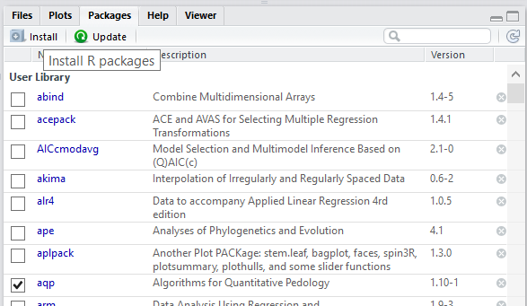
To use a package, you must first install it and then download it. These steps can be done on the command line or using the Packages tab. The following are examples of both methods. R packages are installed only once (until R is upgraded or reinstalled). Each time you start a new R session, you must download the package that you want to use in that session.
In the Packages tab, you will see a list of all the packages installed on your computer and 2 buttons titled “install” or “update”. To install the new package, just select the Install button. You can enter one or more packages while separating a comma.

Use the following commands to find out what packages are installed on your computer:
library ()
# or
installed.packages ()
A very useful package for soil scientists is the soiltexture package, which, as you would expect, allows you to draw soil texture triangles. If you have not already downloaded this package, the following command shows how to install it:
# CRAN (static version)
installed.packages (c (“aqp”, “soilDB”, “soilReports”, “soiltexture”))
# GitHub (development version)
devtools :: install_github (“ncss-tech / soilDB”, dependencies = FALSE, upgrade_dependencies = FALSE, build = FALSE)
2-4-4 Loading packages
After installing the package, it must be loaded in session R to be used.

library (soiltexture)
By checking the box next to the package name, you can download packages using the Packages tab. The soiltexture package documentation of the help functions is available in R.
help (package = “soiltexture”)
This help command sends you to a web page. Scroll down and select the “TT.plot” link. This link displays a web page with instructions on how to use the TT.plot () function in R.
The main application of TT.plot () is the TT.plot (class.sys) function, tri.data. The “class.sym” argument specifies a string of characters that names the text classification system.
# Copied from soiltexture vignette
# Create a dummy data frame of soil textures:
example <- data.frame (
CLAY = c (05,60,15,05,25,05,25,45,65,75,13,47),
SILT = c (05,08,15,25,55,85,65,45,15,15,17,43),
SAND = c (90,32,70,70,20,10,10,10,20,10,70,10),
OC = c (20,14,15,05,12,15,07,21,25,30,05,28)
)
TT.plot (class.sys = “USDA-NCSS.TT”, tri.data = example)

7-4 script writing
RStudio source tabs work as an internal text editor. Commands are usually written (or scripted) before using the R functions in the console. Scripting is basically showing your work. The sequence of functions needed to complete a task in order to document or automate a scripted task. Although scripting may be cumbersome at first, it can save time in the long run, especially for repetitive tasks. Benefits include:
- Allows others to produce your work, which is the foundation of science
- Acts as instructions / reminders on how to do a task
- Enables fast repetition, which saves time and evaluates gradual changes
- Reduces the likelihood of human error
1-7-4 Basic tips for scripting
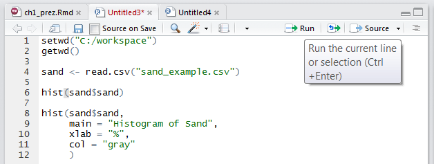
To write a script, just open a new R script file by clicking File> New File> R Script. In the text editor, type a sequence of functions.
- Put each function (eg read.csv ()) on a separate line.
- If a function has a long list of arguments, put each argument on a separate line.
- You can delete a command from the text editor by placing the cursor on a line and typing Crtl + Enter, or by clicking the Run button.
- You can delete a complete R script file by clicking the Source button.
8-4 Save R files
In R you can save several types of files to track what you do. File types include: workspace, scripts, history and graphics. It is important to save often because R, like any other software, may crash periodically. Such problems are especially common when working with large files. You can save your workspace in R via the command line or File menu.
1- 8-4 script .R) R)
The R script is simply a text file of the R commands you typed.
You may want to save your scripts (whether written in R Editor or another program such as Notepad) so that you can refer to them in the future, edit them, and keep track of your tasks. To save R scripts in RStudio, just click the save button from the R script tab. Save scripts with a .R extension. R assumes that script files are saved with only that extension. If you use another text editor, you will no longer have to worry about storing your scripts in R. You can open text files in the RStudio text editor, but be careful to copy and paste Word files, as explained below.

Click the file icon to open the R script.

1-1-4-4 Notes on Word files
It is generally a bad idea to use Microsoft Word to write or save R scripts. Some keyboard characters, such as quotes, are not stored uniformly in Word (for example, “vs.”). The difference is largely indistinguishable to the human eye, but will not work in R.
2-8-4 workspace (.Rdata)
The R workspace (or workspace) contains all the data objects that you have created or loaded in your R session. When you turn off R by typing q () or exiting the application window, it asks you to save your workspace. If you select yes, R saves a file named .RData to its work directory. The next time you open R and reload your .Rdata workspace, all your data objects will be available in R, and all the commands you typed can be used using the up and down arrow keys on the keyboard. Are accessible. You can also save or upload your workspace from the menu at any time from your R session by clicking Session> Save Workspace As .. or click the save button on the Environment tab.

R command to save your workspace:
save.image (file = ”workspace.RData”)
3-8-4 History of R (.Rhistory)
The R history file is a copy of all your keystrokes. Like the R file, the Rhistory file is a text file that lists all the commands you have executed. Does not record a record of results. Click the Open File or Save button to load or save the R history from the History tab. If you download the Rhistory file, your previous commands will be available again with the up and down arrow keys.
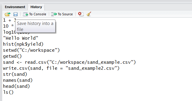
You can also use the command line to load or save your history.
savehistory (file = “sand.Rhistory”)
loadhistory (file = “sand.Rhistory”)
history (max.show = Inf) #displays all previous commands
4-8-4 Graphics R
Graphic outputs can be stored in various formats.
| format | Function |
| pdf (“graphic.pdf”) | |
| Windows metafile | win.metafile (“graphic.wmf”) |
| png | (“Graph.png”) png |
| jpeg | (“Graph.jpg”) bmp |
| bmp | (“Graph.ps”) postscript |
| postscript |
To save the chart: (1) Click on the Plots Tab window 2) Click the Export button, 3) Select the format you want (3) Change the export settings to your liking, and (4) Click Save.

R command to save a chart:
png (file = “npk_yield.png”)
plot (npk $ yield)
dev.off ()
The first line of this command creates a blank file called sand with the JPEG extension. The second line draws the data object from which you want to create a graph (here is the JPEG file that we are creating). The third line closes the graphics device.
5- Rcmdr (Commander R): Graphical user interface for R
While we recommend using RStudio for some of the above reasons, many newcomers to R can benefit from a graphical user interface (GUI) that allows the user to use basic functions. Run from a point and click interface. Fortunately, R for Beginners has R Commander (Rcmdr) GUI, which is similar to JMP. Rcmdr was created by John Fox for his elementary statistical students so that they can see how the software works without having to learn a lot of function names and arguments. Rcmdr is a great way to get acquainted with R and statistics in a GUI environment.
Rcmdr can be opened quickly by entering the following command in console R.
install.packages (Rcmdr)
library (Rcmdr)

