blog posts

When we think of a dynamic programming problem, we must understand the subproblems and how they relate to one another. In this article, we will review dynamic programming.

Algorithms and data structures are integral components of data science. However, most data scientists do not adequately cover the analysis and design of algorithms in their studies. These topics are quite important, and not only data scientists but also programmers should have accurate and complete information about designing algorithms, especially dynamic programming.

In topics related to computer science and statistics, Poil planning and programming efficiently solve search and optimization problems using the two features of overlapping subproblems and optimal infrastructure.

Unlike linear programming, there is no standard framework for formulating dynamic programming problems. More specifically, the dynamic planning concept provides a general approach to solving these issues.

In each case, specialized mathematical equations and relations must be developed to match the problem’s conditions.

What is Dynamic Programming?

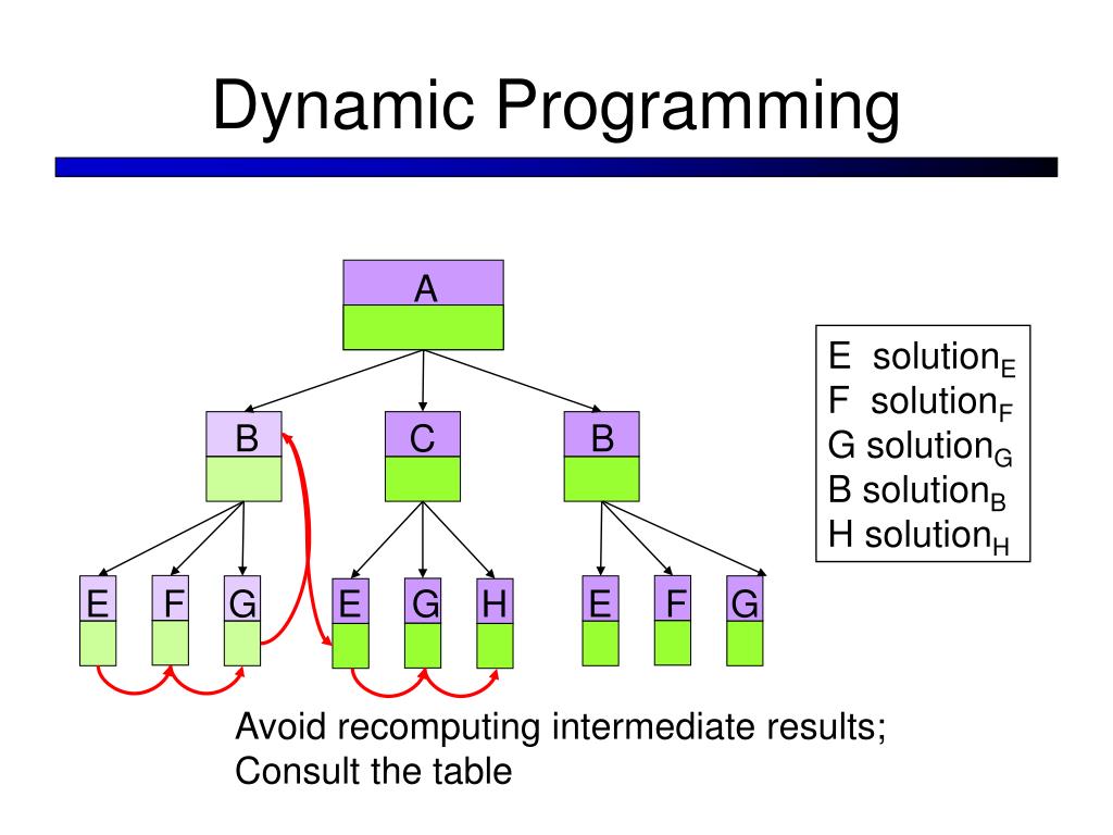
Dynamic programming often stores results in an array for reuse and solves subproblems partially. In this case, the subproblems consisting of only two matrices are first calculated.

Then, the sub-problems consisting of three matrices are calculated. These sub-problems are broken down into two matrices that have already been calculated, and the results are stored in an array.

As a result, they do not need to be recalculated. Similarly, in the next step, the subproblems are calculated with four matrices, and so on. Dynamic programming, like the division-and-conquer method, solves problems by combining the answers to subproblems.

The division-and-solution algorithm divides the problem into independent subproblems. After solving the subproblems recursively, it combines the results and obtains the answer to the main problem.

More specifically, dynamic programming can be used in cases where the subproblems are not independent, that is, when the subproblems themselves have several identical subproblems.

In this case, the division-and-solution method performs more calculations than necessary by repeatedly solving the same sub-problems. A dynamic scheduling algorithm stores sub-problems once and their answers in a table, preventing them from being repeated when they need to be answered again.

What are the hallmarks of dynamic programming?

To use dynamic programming for an issue, it must have two key characteristics: an optimal substructure and overlapping subproblems. Solving a problem by combining the optimal solutions of overlapping subproblems is called “division and solving.” This is why fast, integrated sorting is not considered a dynamic programming problem.

The key to dynamic programming is the principle of optimality. If the parentheses of the whole phrase are to be optimized, the parentheses of the subproblems must also be optimal. That is, the problem’s optimality requires the subproblems’ optimality.

So you can use dynamic programming. The optimal solution is the third step in developing a dynamic programming algorithm for optimization problems. The Development steps of such an algorithm are divided into three parts.

Not all optimization problems can be solved using dynamic programming, because the optimization principle must apply. The principle of optimality applies to a problem if an optimal solution for an instance of the situation always contains the optimal solution for all subsets.

Optimal binary search trees

A binary search tree is a binary tree of elements called keys. Each node contains a key. The keys in the left subtree of each node are less than or equal to the key in that node, and the keys in the right subtree of each node are larger. Or equal to the key of that node

Optimal infrastructure

Optimal infrastructure means that an optimization problem can be solved by combining the optimal solutions of its subproblems. Such optimal infrastructures are usually obtained with a recursive approach; For example, in the Graph (G = (V, E), the shortest path m from vertex A to vertex B shows the optimal infrastructure: Consider every middle vertex of path m.

If m is really the shortest path, then it can be considered two sub-paths, M1 from A to C and M2 from C to B, so that each of these is the shortest path between the two ends (in the same way as cutting and pasting the book Introduction to Algorithms).

The answer can be expressed recursively, just like the Bellman-Ford and Floyd-Warshall algorithms.

Using the optimal infrastructure method means breaking the problem into smaller sub-problems, finding the optimal solution for each sub-problem, and obtaining the optimal solution to the whole problem by combining these partial optimal solutions.

For example, when solving the problem of finding the shortest path from one vertex of a graph to another, we can obtain the shortest route to the destination from all adjacent vertices and use it for a general answer.

In general, problem-solving with this method includes three steps: breaking the problem into smaller parts, solving these sub-problems by breaking them backward, and using partial answers to find the general answer.

The sub-problem graph contains the same information for an issue.

Figure 1 shows the sub-problems of the Fibonacci sequence. Sub-Problem Graph: A directional graph consists of one vertex for each distinct sub-problem, and in the case of a directional edge from the vertex of Graph-problem x to the vertex of sub-problem y, it directly requires an optimal solution for sub-problem x to determine an optimal solution for sub-problem y. y have.

For example, the subproblem graph has an edge from x to y if a top-down recursive procedure for solving x calls itself directly for solving y.

A graph problem can be considered a reduced version of the recursive tree for the top-down recursive method. In this method, we unite all the vertices of a subproblem and orient the edges from parent to child.

The bottom-up method for dynamic programming considers the outline of the subproblem in such a way that all adjacent subproblems of a subproblem are solved first.

In a dynamic bottom-up programming algorithm, we consider the outline of the subproblems to be the “topologically ordered inverse” or “inverted topologically invested subset of the problems.”

In other words, no subproblem is considered until all the subproblems it depends on have been resolved.

Similarly, the top-down (along with memorization) approach to dynamic programming can be seen as an in-depth graph search of sub-problems.

The graph size of the subproblems can help us determine the execution time of the dynamic programming algorithm. Since we solve each subproblem only once, the execution time equals the total number of times it is solved.

The time to calculate the answer to a subproblem is proportional to the degree of the corresponding vertex in the graph, and the number of subproblems is equal to the number of graph vertices.

For example, a simple function implementation of the nth Fibonacci number could be as follows.

function fib (n)

if n = 0

rGraph 0

if n = 1

return 1

return fib (n – 1) + fib (n – 2)

One of the most widely used and popular methods for designing algorithms is Dynamic Programming.

This method works like the divide-and-conquer method, which divides the problem into subproblems. But there are significant differences. When a problem is divided into two or more sub-problems, two situations can occur:

The data of the subproblems have nothing in common and are entirely independent. An example is sorting arrays using the merge or fast method, which divides the data into two parts and arranges them separately.

In this case, the data of one section has nothing to do with the data of the other section, and as a result, the result of that section does not affect the other. The division and solution method usually works well for such problems.

The data in the sub-issue are related or shared. In this case, the so-called subproblems overlap—a clear example is calculating the nth Fibonacci number.

Dynamic programming methods are often used for algorithms that seek to solve problems optimally.

In the method of division and domination, some smaller sub-problems may be equal, in which case they are repeatedly solved, which is one of the method’s disadvantages.

Dynamic programming is a bottom-up method, meaning we solve more minor problems first and then move on to more significant ones.

Structurally, the method of division and domination is top-down; that is, logically (not practically), the process starts with the initial problem and proceeds to solve more minor issues.

FAQ