The Decision Tree is one of the most important and widely used methods in data science for decision-making and prediction problems.

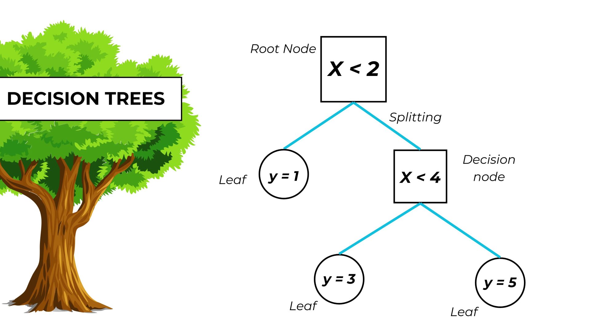
Additionally, decision trees are also used for classification tasks. In a decision tree, nodes are interconnected, and each one contains a condition. This condition is based on one or more features from the input data.

In simple terms, a decision tree consists of a series of nodes where each node represents a condition, and its branches represent different decisions. Based on the inputs and existing rules, the decision tree follows a path to reach a final decision.

How Do We Build a Decision Tree?

In general, a decision tree is a powerful tool used in data analysis and complex decision-making. In some cases, due to its simple structure, a decision tree performs better than more complicated models used for decision-making and prediction. A decision tree is composed of nodes and branches.
Each node describes a state that is connected to other nodes, called branches. The branches represent different decisions made under various conditions. When it comes to building a decision tree, we face a set of steps that must be followed carefully to draw the tree accurately. These steps are as follows:

1. Feature Selection Feature Selection means choosing a set of variables that provides us with the most information for deciding a problem. The main goal of feature selection is to reduce the dimensionality of the data and increase the model’s efficiency and accuracy.
By removing or selecting certain features, we can eliminate unnecessary items and improve the model’s performance. Various methods are available for feature selection, some of which are:

• Filter-based Methods: In these methods, features are evaluated based on statistical criteria such as their correlation with the target variable (mutual information), variance, or hypothesis testing. Features with the highest relevance and importance to the target variable are selected.
• Wrapper Methods: These methods use machine learning algorithms to evaluate the quality of features. A subset of features is selected, the model is trained using them, and then its performance is evaluated using a metric like accuracy or prediction error. This process is repeated iteratively to find the best subset of features.
• Embedded Methods: In these methods, feature selection is performed directly within the model learning process. In the decision tree model, for each node, a feature is selected based on a criterion like information gain or the Gini coefficient to best split the data.

2. Structuring the Tree After splitting the data, the decision tree is built as a hierarchy of nodes. Each node has a specific feature, and its children represent the possible values of that feature. This process continues until the data is completely separated or a stopping condition is met (such as a specified maximum tree depth).

3. Labeling After structuring the tree, labels (classes or target values) are assigned to the leaf nodes. This way, the decision tree is trained and ready to be used for predicting and classifying new data.

4. Prediction Prediction means using the constructed tree to predict or classify new data. After building the decision tree and labeling the leaf nodes, it can be used to predict and classify new samples. For example, suppose a decision tree is built that classifies people into “Buyer” and “Passerby” categories based on features like age, gender, and employment status.
Now, if a new sample with features like age 30, male gender, and “employed” status enters the tree, the tree will predict, based on its decision rules, that this sample belongs to the “Buyer” category.

What are the Advantages of Using a Decision Tree in Data Science?

The decision tree is one of the essential models in data science, and as mentioned, it is easier to understand compared to some other standard models. Some of the advantages of a decision tree are:

• Interpretability: Due to its hierarchical and understandable structure, a decision tree is highly interpretable. You can easily understand how the tree’s decisions are made based on features and rules.
• Usability for Classification and Prediction: A decision tree can be used for both classification and prediction problems. We can assign samples to different categories or assign labels to new data.
• Fast Processing: Due to its simple structure and independence from training data during prediction, a decision tree has a rapid execution time. Comparison and decision-making for each node are based on a small number of features, which significantly increases the speed of predicting new data.
• Ability to Handle Numerical and Categorical Features: A decision tree can work with both numerical and categorical features. For numerical features, criteria like the mean can be used to split data, while for categorical features, the available values can be used for splitting.
• Robustness to Missing Data and Noise: A decision tree is highly robust to noisy and incomplete data because its operation is based on splitting and distinguishing data from one another. Therefore, a change in a single sample or feature has little effect on the tree’s overall performance.
• Ability to Identify Important Features: By splitting data based on features, a decision tree can identify key features in the data. By examining the tree’s structure and the placement of features within it, one can understand which features play the most significant role in decision-making.
• Data Analysis: A decision tree helps us analyze data comprehensively. By examining the features and various conditions in the tree, we can identify and extract patterns, relationships, and essential features in the data.

What Algorithms are Available for Building a Decision Tree in Data Science?

Data scientists use various algorithms to build decision trees. Some of the most famous algorithms in this field are:

• ID3 Algorithm: The ID3 algorithm is one of the well-known methods for building a decision tree. This algorithm uses the Information Gain approach. It works by first selecting features that are worthy of being the root. To choose the optimal feature, the information gain criterion is used. In the next step, the data is split based on the different values of this feature into corresponding sub-nodes. The above steps are repeated for each sub-node. For each sub-node, the feature with the highest information gain is chosen as its root, and the data is split accordingly. This process continues until a stopping condition is met, for example, when all data in a sub-node is of the same class or all features have been used. When a stopping condition is met, a label (the majority label in the data) is assigned to the leaf node.
• C4.5 Algorithm: This is another famous algorithm for building decision trees, which is an improved and generalized version of ID3. It introduces changes in feature selection methods and tree geometry. The process of creating a tree with C4.5 is almost similar to ID3. It uses information gain to select the root feature, but C4.5 also uses another criterion called Gain Ratio to counter the problem of bias towards features with a large number of values. Ultimately, the feature with the highest Gain Ratio is chosen as the root. Other steps are similar to the ID3 algorithm.
• CART Algorithm: This algorithm is used for classification and regression. CART trees are divided into classification trees and regression trees. The CART algorithm works similarly for building both types of trees, with the difference that in classification trees, the outputs are class labels. In contrast, in regression trees, the outputs are continuous values. The process starts with selecting a feature and a split point. At each step, based on an optimization criterion, a feature and a divided value for that feature are chosen. Standard criteria include the Gini Index for classification trees and Mean Squared Error for regression trees. The algorithm selects the feature and split value by trying to reduce error or increase class purity. Next, the data is split into sub-nodes based on the chosen split value. These steps are repeated for each sub-node until a stopping condition is met, such as a minimum number of samples in a node, a specified tree depth, or the creation of pure leaves.
• Random Forest Algorithm: Random Forest is a user-friendly machine learning algorithm that often yields good results even without hyperparameter tuning. Due to its simplicity and versatility, it is used for both classification and regression. Random Forest is a supervised learning model that maps data to outputs during the training phase. Historical data relevant to the problem domain, along with the correct value the model should learn to predict, are fed to the model. The model learns the relationships between the data and the values the user wants to predict.
• XGBoost Algorithm: This is an algorithm used for prediction and data analysis. By using Gradient Boosting and an optimized use of decision trees, this algorithm provides a robust and accurate model for complex problems.

How to Use a Decision Tree in Data Science?

The decision tree is an essential and influential method in the field of data science and can be widely used in many problems. Some of the main applications are:

• Data Classification: Decision trees are well-suited for data classification problems. Using the features of the data, a decision tree can divide the data into different categories and predict classification labels for them. This is used in problems like spam email detection, disease diagnosis, financial decision-making, and customer segmentation.
• Prediction and Regression: Using data features, a decision tree can predict numerical values. For example, it can be used to predict house prices based on related features like square footage, number of rooms, and geographical location.
• Feature Selection: A decision tree can be used as a tool for feature selection in data-driven problems. By analyzing the structure of the decision tree, one can identify key features in prediction and classification and use them to build more efficient models.
• Explaining Decision Rules: One of the advantages of a decision tree is that it provides understandable and explainable decision rules. By analyzing the tree structure and different paths, one can extract and explain the decision rules clearly and concisely.

Example of Implementing a Decision Tree in Python

Now, let’s practically demonstrate how to implement a decision tree in Python for a weather data classification problem. In this example, we will use features like temperature, humidity, and wind speed to predict the next day’s weather.

Translator’s Note: The original text describes a “weather” dataset but uses the datasets.load_iris() function from Scikit-learn, which loads a famous dataset for classifying iris flower species. The code will run correctly with the Iris dataset, but the variable names and comments reflect the Iris data, not weather data.

from sklearn import datasets
from sklearn.model_selection import train_test_split
from sklearn.tree import DecisionTreeClassifier
from sklearn import metrics

# Load the Iris dataset
# The original text mistakenly refers to this as a weather dataset.
iris_data = datasets.load_iris()

# Separate features and labels
X = iris_data.data
y = iris_data.target

# Split data into training and testing sets
X_train, X_test, y_train, y_test = train_test_split(X, y, test_size=0.2, random_state=1)

# Create a Decision Tree Classifier model with default parameters
clf = DecisionTreeClassifier()

# Train the model with the training data
clf.fit(X_train, y_train)

# Predict labels for the test data
y_pred = clf.predict(X_test)

# Evaluate the model's accuracy
accuracy = metrics.accuracy_score(y_test, y_pred)
print("Model Accuracy:", accuracy)

In this example, the Scikit-learn library is used. First, the dataset is loaded using datasets.load_iris. Then, the features and labels are separated. Next, the data is split into training and test sets using train_test_split. Here, 80% of the data is used for training and 20% for testing.

Then, a decision tree model is createdDecisionTreeClassifier, and the model is trained on the training data. The predicted labels for the test data are calculated using predict. Finally, the model’s accuracy is calculated and displayed using accuracy_score the Scikit-learn library.

How Can We Add Different Parameters to the Model?

In the Scikit-learn Decision Tree model, you can adjust the model’s behavior and performance using various parameters. Below are some important parameters that allow you to adapt the model to your needs and the problem’s settings.

• criterion: This parameter specifies the criterion used to measure the quality of a split. For classification problems, gini they  entropy are commonly used. The default is gini.
• max_depthThis parameter specifies the maximum depth the tree can have. By setting this parameter, you can prevent overfitting. If you set this parameter toNone, the tree will expand until all leaves are pure. The default is None.
• min_samples_split: This parameter specifies the minimum number of samples required to split an internal node. If the number of samples in a node is less than this value, no further splitting occurs. This parameter helps prevent overfitting. The default is 2.
• min_samples_leafThis parameter specifies the minimum number of samples required to be at a leaf node. A split point at any depth will only be considered if it leaves at least min_samples_leaf training samples in each of the left and right branches. This is also useful for preventing overfitting. The default is 1.
• max_featuresThis parameter determines the number of features to consider when looking for the best split. You can set this to an integer, a float (fraction), or ‘auto’/’sqrt’/’log2’. The default is None (all features are considered).
• splitterThis parameter determines the strategy used to choose the split at each node. Possible values are best (to select the best split) and random (to choose the best random split). The default is best.
• random_state: This parameter is used for controlling the randomness of the estimator. By setting a fixed number, the model will be generated with the same sequence of data and random splits every time.
• class_weight: Using this parameter, you can assign different weights to the classes. This is useful for dealing with imbalanced class problems.

Final Analysis

This document provides an excellent and thorough introduction to the Decision Tree algorithm, suitable for beginners in data science. It systematically covers the topic from foundational concepts to practical implementation, making it a valuable educational resource.

Strengths of the Text:

• Comprehensive Coverage: The text is well-structured, guiding the reader through the entire lifecycle of a decision tree model: its conceptual basis, the step-by-step construction process (feature selection, structuring, labeling), its advantages, and its primary applications.
• Detailed Algorithmic Overview: A significant strength is the detailed explanation of key tree-building algorithms like ID3, C4.5, and CART. It correctly highlights the specific splitting criteria (Information Gain, Gain Ratio, Gini Index) that differentiate them. The inclusion of more advanced ensemble methods like Random Forest and XGBoost provides valuable context, showing how single decision trees serve as building blocks for more powerful models.
• Clarity and Interpretability: The document effectively emphasizes one of the decision tree’s main selling points: its high interpretability. The clear, rule-based structure is explained well, making it obvious why this model is often preferred for tasks requiring transparency.
• Practical Implementation: The inclusion of a Python code example using the popular Scikit-learn library is a significant plus. It grounds the theoretical concepts in a real-world application, demonstrating how easily a model can be built, trained, and evaluated. The final section on hyperparameter tuning (max_depth, min_samples_split, etc.) is also highly practical, introducing the reader to the crucial concept of model optimization and preventing overfitting for Improvement:

• Factual Error in Example: The most notable weakness is the factual error in the Python example, where a “weather classification” problem is described, but the code implements the load_iris() Dataset. While this doesn’t affect the code’s functionality, it can be confusing for a learner. A more appropriate dataset would have strengthened the example’s coherence.
• Discussion on Overfitting: While the text mentions that hyperparameter tuning can prevent overfitting, it could benefit from a more explicit discussion of why single decision trees are particularly prone to this issue. This would create a stronger narrative for why methods like pruning and ensemble models (e.g., Random Forest) were developed and are often necessary.

Conclusion:

Overall, this is a high-quality, well-written guide to decision trees. It successfully balances theoretical depth with practical application. Despite the minor error in the code example, the document serves as a valuable and comprehensive primer for anyone to understand and utilize decision tree models in data science.