A Probability Distribution Is A Function That Assigns Different Values ​​Of A Random Variable To Specific Probabilities.

In Other Words, The Probability Distribution Specifies The Probability That Each Possible Value Of A Random Variable Will Occur.

A probability distribution can be defined as a probability function or density function.

Probability distributions are important in probability, statistics, and other fields dealing with random phenomena. For example, in engineering, probability distributions can describe and predict the behavior of complex systems such as power grids, traffic systems, etc.

In the life sciences, probability distributions can describe and predict the behavior of cells, the immune system’s response to diseases, etc.

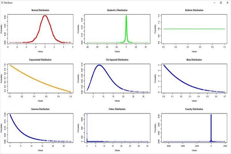
Many probability distributions exist, including regular, binomial, Poisson, etc. Each of these distributions has its characteristics specifically used to describe different data.

In Python, to work with probability distributions, there are various libraries, some of which are as follows:

NumPy

This library is optimized for working with large arrays and mathematical operations. NumPy includes functions for working with probability distributions such as the standard, uniform, and beta distributions. NumPy contains parts for working with probability distributions. You must first add NumPy to your Python code to use these functions. To do this, put the following code at the beginning of your code:

import numpy as np

Now you can use NumPy functions to work with probability distributions. For example, you can use the `np.random.normal()` function to generate random samples from a normal distribution. This function works as follows:

Np. random.normal(loc=0.0, scale=1.0, size=None)

Here, `loc’ is the mean of the normal distribution, `scale’ is the standard deviation of the normal distribution, and `size’ is the number of random samples. For example, you could generate 1000 random samples from a normal distribution with a mean of 2 and a standard deviation of 3:

samples = np. Random.normal(loc=2.0, scale=3.0, size=1000)

NumPy also includes functions for working with various other probability distributions. For example, you can use the `np.random.uniform()` process to generate random samples from the uniform distribution and the `np.random.poisson()` position to create random samples from the Poisson distribution.

SciPy

This library is optimized for scientific and engineering operations and includes functions for working with probability distributions such as every day, uniform, and beta distribution. Also, SciPy contains procedures for performing statistical data analysis, such as linear regression and factor analysis. SciPy is one of the most widely used Python libraries for working with probability and statistical distributions. You must first add SciPy to your Python code to use this library. To do this, put the following code at the beginning of your code:

Import script. Stats as stats

Now you can use SciPy functions to work with probability distributions. For example, you can create a normal distribution object using the `stats. Norm ()` function. This function works as follows:

stats.norm(loc=0.0, scale=1.0)

Here, `loc’ is the mean of the normal distribution, and `scale’ is the standard deviation of the normal distribution. For example, you could create a normal distribution with a mean of 2 and a standard deviation of 3:

normal_dist = stats.norm(loc=2.0, scale=3.0)

Now you can use the functions of this object to calculate different values ​​such as probability density function, cumulative distribution function, and different percentage values. For example, you can calculate the probability density function at point 4:

pdf_value = normal_dist.pdf(4)

Similarly, you can calculate the cumulative distribution function in point 3:

cdf_value = normal_dist.cdf(3)

Also, SciPy includes functions for working with various other probability distributions. For example, you can use the `stats. Uniform ()` process to create a uniform distribution object and the `stats. Poisson ()` function to create a Poisson distribution object.

Pandas

This library is optimized for working with tabular data and includes functions for probabilistic distributions such as regular and beta distributions. Pandas is one of the most widely used Python libraries for working with tabular data.

This library contains functions for data loading, transformation, analysis, etc. To use Pandas to work with possible distributions, you must first add Pandas to your Python code. To do this, put the following code at the beginning of your code:

Import pandas as pd

Now you can use Pandas to load tabular data and analyze it. For example, you can read a column from a data table as a probability distribution. First, load the data table and convert the desired column to a NumPy array. Then, you can use NumPy and SciPy functions to work with probability distributions.

For example, suppose you want to read the “age” column from a data table as a normal distribution. First, load the data table:

data = pd.read_csv(‘data.CSV)

Next, convert the “age” column to a NumPy array:

age_array = data[‘age’].values

Now you can use NumPy and SciPy functions to work with probability distributions. For example, you can create a normal distribution object using the mean and standard deviation of the “age” column:

From scipy.stats import norm

age_mean = age_array.mean()

age_std = age_array.std()

age_dist = norm(loc=age_mean, scale=age_std)

Now you can use the functions of this object to calculate different values ​​such as probability density function, cumulative distribution function, and different percentage values. For example, you can calculate the probability density function at point 40:

pdf_value = age_dist.pdf(40)

Similarly, you can calculate the cumulative distribution function at point 30:

cdf_value = age_dist.cdf(30)

Scikit-learn

This library for machine learning includes various algorithms for working with probability distributions such as Gaussian distribution, beta distribution, and Poisson distribution. Scikit-learn is one of the most widely used Python libraries for machine learning.

This library includes functions for implementing machine learning algorithms, data preprocessing, model evaluation, etc. To use Scikit-learn to work with probability distributions, you can use functions like `KernelDensity.’ First, you need to add Scikit-learn to your Python code. To do this, put the following code at the beginning of your code:

From sklearn.neighbors import KernelDensity

Now you can use KernelDensity to estimate the probability distribution of your data. For example, suppose you want to estimate the probability distribution of the data in the “age” column of a data table. First, load the data table:

import pandas as pd

data = pd.read_csv(‘data.CSV)

Next, convert the “age” column to a NumPy array:

age_array = data[‘age’].values.reshape(-1, 1)

Here, the `reshape` function is used to reshape the array to a shape suitable for use in `KernelDensity.`

Now you can create a kernel density object using the Gaussian kernel model:

kde = KernelDensity(kernel=’gaussian’, bandwidth=0.5).fit(age_array)

Here, `kernel’ is the kernel model type, and `bandwidth’ is the bandwidth parameter.

Now you can use the function `score_samples’ to calculate the value of the logarithm of the probability distribution of arbitrary data. For example, you can calculate the value of the logarithm of the probability distribution at point 40:

import numpy as np

log_pdf_value = kde.score_samples(np.array([[40]]))

pdf_value = np.exp(log_pdf_value)

Similarly, you can calculate the value of the logarithm of the probability distribution at point 30:

log_cdf_value = kde.score_samples(np.array([[30]]))

cdf_value = np.exp(log_cdf_value)

Note that `score_samples’ functions return the value of the logarithm of the probability distribution, so you must use the `exp’ function to calculate the value of the probability distribution.

PyMC3

This library is optimized for probabilistic modeling and includes functions for working with probabilistic distributions such as the standard, uniform, beta, and Poisson distributions. PyMC3 is an open-source library for performing probabilistic programming based on Python. This library provides facilities for defining and running probabilistic models, performing MCMC sampling, evaluating models, etc.

To use PyMC3 to work with probability distributions, you can use functions like `Normal’ and `Uniform.’ First, you need to add PyMC3 to your Python code. To do this, put the following code at the beginning of your code:

Import pymc3 as pm

Now you can use PyMC3 to define a probabilistic model. For example, suppose you want to estimate the probability distribution of the data in the “age” column of a data table. First, load the data table:

import pandas as pd

data = pd.read_csv(‘data.CSV)

Next, define the “age” column as a random variable in PyMC3:

With pm.Model() as age_model:

age_mean = pm.Uniform(‘age_mean’, lower=0, upper=100)

age_std = pm.Uniform(‘age_std’, lower=0, upper=50)

age_dist = pm.Normal(‘age_dist’, mu=age_mean, sd=age_std, observed=data[‘age’])

Here, `Uniform’ is used to define a uniform distribution. Also, `Normal’ describes a normal distribution with mean `age_mean’ and standard deviation `age_std.’ “observed” is provided as input data to the model.

Now you can use the `sample` function to run MCMC sampling on the model:

with age_model:

trace = pm.sample(1000, chains=1, tune=1000)

Here, the number of samples from the model is given as the first parameter to `sample.` Also, by specifying the “chains” parameter, the number of MCMC chains is determined. The `tune’ parameter is also the number of samples to be sampled to tune the MCMC parameters automatically.

Now you can use the obtained samples to calculate different values ​​such as mean and standard deviation:

age_mean_samples After running the sampling, you can use the output in the `trace` variable. For example, you can calculate the mean and standard deviation of the probability distribution of the data in the “age” column using the samples obtained for `age_mean` and `age_std`:

age_mean_samples = trace[‘age_mean’]

age_std_samples = trace[‘age_std’]

mean_estimate = age_mean_samples.mean()

std_estimate = age_std_samples.mean()

Here, by accessing the samples obtained for `age_mean` and `age_std,` the mean and standard deviation of the probability distribution of the “age,” column data are calculated with `mean_estimate` and `std_estimate,` respectively.

Alternatively, using the’ pm,’ you can calculate the probability distribution at arbitrary points. Distributions.Normal. List function. For example, the value of the probability distribution at point 40 can be calculated using the values ​​obtained for `age_mean` and `age_std`:

From scipy.stats import norm

pdf_value = norm(mean_estimate, std_estimate).pdf(40)

The `pdf` function calculates the probability distribution value at point 40. Similarly, you can calculate the cumulative probability distribution at point 30 using the `cdf` function:

cdf_value = norm(mean_estimate, std_estimate).cdf(30)

TensorFlow Probability

This library is optimized for probabilistic modeling and includes functions for working with probabilistic distributions such as the standard, uniform, beta, and Poisson distributions. TensorFlow Probability is an open-source library for probabilistic programming built on top of TensorFlow. This library provides tools for defining and running probabilistic models, performing MCMC sampling, evaluating models, and more.

To use TensorFlow Probability to work with probability distributions, you can use classes like `top.distributions.Normal` and `top.distributions.Uniform`. First, you need to add TensorFlow Probability to your Python code. To do this, put the following code at the beginning of your code:

Import tensorflow_probability as top

Now you can use TensorFlow Probability to define a probabilistic model. For example, suppose you want to estimate the probability distribution of the data in the “age” column of a data table. First, load the data table:

import pandas as pd

data = pd.read_csv(‘data.CSV)

Next, define the “age” column as a random variable in TensorFlow Probability:

Import tensorflow as tf

age_mean = top. Util.TransformedVariable(

initial_value=50., bijector=tfp.bijectors.Softplus(), name=’age_mean’)

age_std = top. Util.TransformedVariable(

initial_value=10., bijector=tfp.bijectors.Softplus(), name=’age_std’)

age_dist = top. Distributions.Normal(loc=age_mean, scale=age_std)

Here, `TransformedVariable` defines random variables with non-linear mapping functions (for example, the Softplus function). Also, `Normal’ describes a normal distribution with mean `age_mean’ and standard deviation `age_std.’

Now you can use the `sample` function to run MCMC sampling on the model:

num_samples = 1000

num_burnin_steps = 500

@tf.function

def run_chain():

samples = top. mcm.sample_chain(

num_results=num_samples,

num_burnin_steps=num_burnin_steps,

current_state=[age_mean, age_std],

kernel=tfp. mcm.HamiltonianMonteCarlo(

target_log_prob_fn=lambda age_mean, age_std: age_dist.log_prob(data[‘age’]).sum(),

step_size=0.05,

num_leapfrog_steps=5),

trace_fn=lambda _, pkr: pkr.inner_results.is_accepted)

return samples

samples = run_chain()

age_mean_samples, age_std_samples = samples

 

Here, the number of samples from the model is specified by `num_samples.` Also, the number of pieces for MCMC parameterization is determined by `num_burnin_steps.` Here, the Hamiltonian Monte Carlo algorithm is used for sampling.

You can get the samples obtained from the model, the mean, and the standard deviation of the “age” column as follows:

mean_age = tf.reduce_mean(age_mean_samples)

std_age = tf.reduce_mean(age_std_samples)

Finally, according to the obtained samples, you can estimate the probability distribution of the “age” column and, for example, calculate the value of P(age > 60):

age_dist = top. Distributions.Normal(loc=mean_age, scale=std_age)

p_age_gt_60 = 1 – age_dist.cdf(60)

Here, `cdf’ calculates the cumulative probability distribution function.

Pyro

This library is optimized for probabilistic modeling and includes functions for working with probabilistic distributions such as the standard, uniform, beta, and Poisson distributions. Pyro is a probabilistic library for Python based on PyTorch. Using Pyro, you can define complex probabilistic models and optimize them using MCMC sampling or gradient-based optimization algorithms.

You must first install the library to use Pyro to define a probabilistic model. To do this, enter the following command in the terminal:

Pip install pyro-ppl

Then, to define a probabilistic model, you can use the following commands:

Import pyro

import pyro. Distributions as dist

def model(data):

# Define model parameters

mu = Pyro.param(‘mu’, torch.tensor(0.))

sigma = Pyro.param(‘sigma’, torch.tensor(1.), constraint=dist.constraints.positive)

# Define a random variable for the data

with pyro.plate(‘data’, len(data)):

x = pyro.sample(‘x’, dist.Normal(mu, sigma), obs=data)

return x

In this code, the `model` function is a PyTorch neural network function that defines a probability distribution over the input data (here, we denote the data as `data`).

This model has two parameters: `mu’ and `sigma,’ defined using the `pyro. Param’ function. Also, using `pyro. Sample’ is a random variable with normal distribution with mean `mu’ and standard deviation `sigma,

To use this model for learning, you can use the Variational Inference algorithm. To do this, run the following commands:

From Pyro. Infer import SVI, Trace_ELBO

from Pyro. optim import Adam

# Definition of the posterior distribution estimation function

def guide(data):

# Define the parameters of the posterior distribution

mu_q = Pyro.param(‘mu_q’, torch.tensor(0.))

sigma_q = Pyro.param(‘sigma_q’, torch.tensor(1.), constraint=dist.constraints.positive)

# Define a random variable for the data

With Pyro.plate(‘data’, len(data)):

pyro.sample(‘x’, dist.Normal(mu_q, sigma_q))

# Define data

data = torch.and(100)

# Definition of the cost function

svi = SVI(model, guide, Adam({‘lr’: 0.01}), loss=Trace_ELBO())

# Model training

for i in range(1000):

loss = svi.step(data)

if i % 100 == 0:

In this code, the `guide` function is a PyTorch neural network function that defines a probability distribution for the `mu` and `sigma` parameters. This posterior distribution is determined using the `Pyro—Param’ process.

In the following, we have defined the data used to train the model using `torch. Rand. Next, we define an SVI object using the “SVI” function, the Trace ELBO cost function, and the Adam optimizer algorithm. Then, using the step function, we train the model based on the input data.

By the end of the tutorial, you can get the following parameter values:

mu_q = Pyro.param(‘mu_q’)

sigma_q = Pyro.param(‘sigma_q’)

Alternatively, you can estimate the probability distribution of the posterior parameters using the following commands:

From Pyro. infer import Predictive

predictive = Predictive(model=model, guide=guide, num_samples=1000)

samples = predictive(data)

mu_samples = samples[‘mu’].detach().numpy()

sigma_samples = samples[‘sigma’].detach().numpy()

mu_mean = mu_samples.mean()

sigma_mean = sigma_samples.mean()

Here, using the “Predictive” function, you can estimate the probability distribution of the posterior parameters. Using `num_samples,’ the number of samples to estimate the probability distribution is specified. Then, using `samples,’ you can get samples from the probability distribution of the posterior parameters. Finally, using `mean,’ we calculate the mean of the probability distribution of the posterior parameters.

last word

These libraries are only part of the libraries available for working with probability distributions in Python. Because there are many libraries, you may use one or more depending on your needs. For example, if you’re looking for a library for probabilistic modeling, PyMC3, TensorFlow Probability, and Pyro are all good choices. However, Pandas is a good choice if you are looking for a library for working with tabular data.

Also, for working with probabilistic distributions, the NumPy library is very widely used, and most other libraries also use NumPy for some of their operations. So, if you are familiar with NumPy, it might be better to use it to work with possible distributions.