


7 Excel Tools For More Productivity
Do You Also Use Excel? Would You Like To Be Able To Separate, Sort And Analyze Your Data On This Platform And Use Them Better?
This article will discuss seven useful tools for easier access to your data in Excel.
Most tools are fairly basic, but some tools may be mediocre. However, with a little practice, anyone can easily use them in Excel.
Sum _
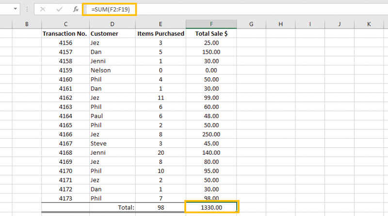
This tool is as simple as it sounds. Use the Sum function, to sum up all the requested data in Excel. You can do this in rows or columns and add multiple number sources together in your spreadsheet.
Let’s take a look at creating a basic Sum formula:
=Sum(value1,value2,value3…)
To summarize a range of data, you replace the value in the formula with the cells. For example, to add cells A1 to A20, use “Sum(A1:A20)”. More cells or ranges can be added with commas “=Sum(A1:A20, B15, C2:C5)”.
You can tell the formula exactly which cells to include by typing in the cell names, or you can click and drag a box over the cells you want to have, and the formula will automatically add them.
You can also choose to collapse at the end of a row or column or create a table elsewhere on your sheet. You can even aggregate the contents of one sheet and have them drag the results to another sheet entirely. Although this tool is simple, it is much more useful than it seems.
COUNT _
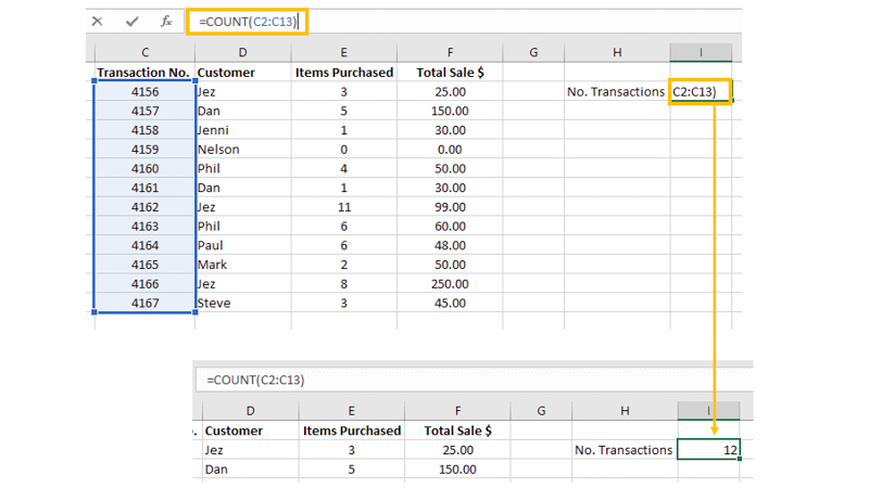
The most basic Count function does exactly what its name suggests. This tool counts the total number of highlighted cells in a range. However, this tool does not sum up the entire contents of the cells, only the number of cells present. We use the following formula in this tool:
=Count(value1,value2,value3…)
You can list the values, cells, or the range of cells you want to include in the parentheses. A coverage can span multiple rows and columns, such as A1:A50 or A1:D50.
The above example shows the total number of customer transactions in a small database.
The count function only counts cells that contain numbers, so if a cell is empty or contains text, it ignores the cell entirely.
COUNTIF
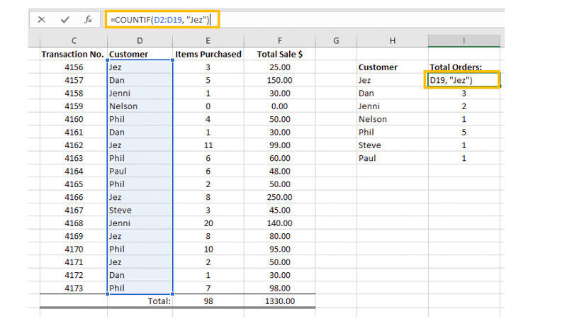
This function in Excel only counts cells if they meet the specified criteria. For example, you may want to count only cells containing a specific name, ID number, or value above or below a certain threshold. So it is better to use this tool.
=CountIf(range,criteria)
We select a range similar to the previous count function, then insert a comma and specify the criteria we want to consider. In the example below, we’ve added the number of orders for each customer by counting the times their name appears in the order list in the model above.
For example, if we want only to count sales above $100, set the formula criteria to >100. To do this, the formula would be “=CountIf(F1:F19, “>100”). Measures can be quite diverse.
SUMIF
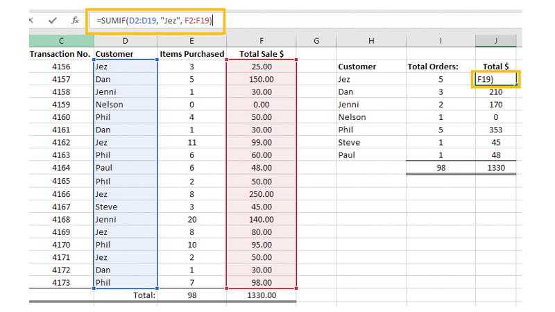
Like CountIf, we can use SumIf only to consider cells that meet our criteria. The difference here is that Countif only counts the number of cells, while SumIf sums the cells if their contents match your instructions.
=SumIf(range,criteria,[sum_range])
With this tool, you can create a whole string of different criteria in Excel, aggregating data into multiple cells that meet your strict rules. One difference in this tool is the inclusion of [sum_range] in the formula. This allows us to specify rules in one column but add values from another corresponding column.
MIN / MAX
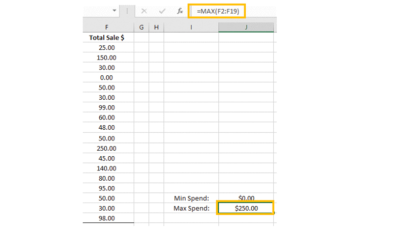
This great Excel tool pulls the highest or lowest values from a set of numbers to save you from going through data lines and spotting the differences. This tool can show you which customers spend the most on your business.
=Min(value1,value2,value3…)
Or
=Max(value1,value2,value3…)
This little tool can be a time saver. As your data changes rank, the min and max tools keep the information up-to-date by constantly looking at the formula and ensuring it’s correct.
You can combine this with multiple conditional formatting to change cells or text to a different color and style or push information to a summary page so you’re always aware of any changes.
RANK _
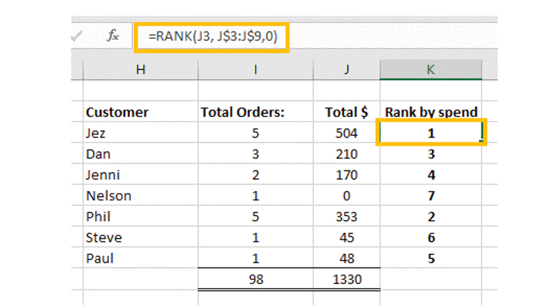
Instead of looking at the highest and lowest values with the Min/Max functions, you can rank a data set based on their values. This is done using the rank formula.
Depending on your data, the rank function can be used to quickly see where you should focus your attention, such as which products are selling the least or which web pages are getting the most clicks.
=RANK(number,ref,[order])
You select the number you want to assign a rank, followed by a “ref,” a group of values the specified number will be compared to, followed by an optional “order” value which can be 0 for descending or 1 to climb.
The example above shows which customers spend the most or the least on sales. Depending on our needs, we can easily look at the sales volume by selecting the previous column.
VLOOKUP
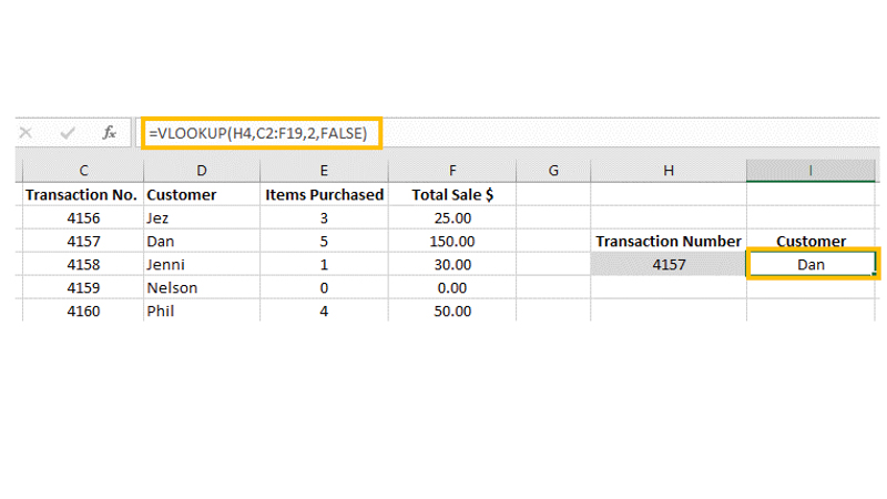
VLookup is a handy tool in Excel, but some people find it difficult to use. By entering a unique value from the first column of your table (such as order number, ID number, or name), the Vlookup function will scan the entire table and return some specific data related to your entry.
Using our customer database from above, we can type in the unique transaction number from the first column to display all the details for that transaction.
The formula used for this is:
=VLOOKUP(lookup_value,table_array,col_index_num,[range_lookup)
Although this tool looks complicated at first, it is quite simple. Let’s break it down:
Lookup_value is the cell that is read before starting the lookup. This is a unique string of information you enter to initiate a search. For example, you enter a transaction number and search for a specific sale for a customer.
The array table or Table_array is the search location. Here you specify which data should be considered in the lookup, and the function will look up this table every time you enter a lookup_value. Your unique lookup_value must always be in the first column of this table.
col_index_num is the column of the above array that provides the data for the output. Your lookup_value finds it in the collection and calls the data in the incoming number column.
Range_lookup is an optional field. You can enter TRUE or FALSE in this field. If TRUE, the search is performed to find an approximate match. If FALSE, the search looks for an exact match. If left blank, it will always default to TRUE.
By extending the Vlookup to more cells, we can create a complete recount of the customer’s completed order with each transaction number. You must change the column number to look at the adjacent information.
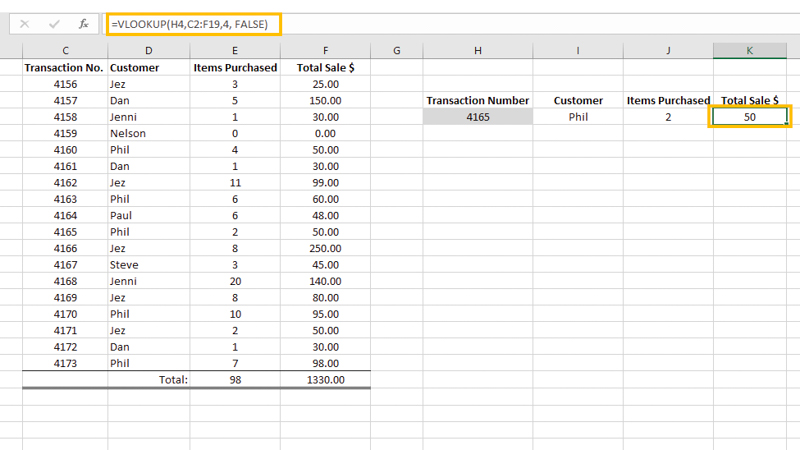
As useful as Vlookup tools are, they also have several limitations.
First, the VLookup value will not detect any duplicate values. If two transactions have the same ID number, this function finds the first occurrence and stops. That’s why it’s important to have a unique value. For example, if we used last names and had 2 Smiths, Vlookup would always stop at the first Smith.
Second, Vlookup can only search to the right. This function looks in the left column for “Lookup_value” and then returns information from the right columns (as specified by the user). Of course, other tools exist to solve this problem, such as the XLOOKUP function, but they are a little more advanced.