blog posts

It is rare to find a brand or a company like Google that has penetrated so much in all aspects of human life or, better said, has served humanity. One of the essential service packages of this company in recent years is Google Workspace. This software product includes several other web applications, Google Sheets being one of them.

The range of Google Sheet users ranges from students and teachers to commercial companies and even government organizations. This software is an excellent tool for storing and managing data with the ability to work simultaneously, share, and write formulas. Google Sheets training is essential for this software’s optimal, fast, and maximum use. The simple user interface of this software also makes it easy to learn.

This article teaches the most essential methods of using Google Sheets. Before that, however, we need to review the benefits of using this software. If you are a student, teacher, employee, or business owner, join us, and from now on, organize and share your data optimally and for free.

What are the Advantages of Using Google Sheets?

 

Most of us are familiar with Microsoft’s Excel program. Introduced in 1987, the software has been popular with users of digital data, from students to business executives and scientists. But this program, like any other offline software, had a fundamental weakness: the inability to share or work on data simultaneously. This need has been felt increasingly in the last decade, especially in a world where people work on a project from different parts of the world. Google entered the competition with Microsoft with its Google Sheet software 2012 to cover this weakness.

• Microsoft Introduced Its Own Version Of Linux

Google Sheets is a web-based software that automatically stores data on virtual servers. Therefore, it is possible to access a file from anywhere and at any time only by having a digital device. This software is considered a collaborative tool that enables the owner of the File to give access to others using their Jamil accounts at the following levels:

• View or View
• Editing or Edit
• Commenter
• Ownership

Other general and essential advantages of Google Sheets include the following:

• Free and easy access that only requires a Google or Gmail account.
• Excellent compatibility with all digital devices, from mobile phones and tablets to laptops and various operating systems
• Excellent computational, analytical, scheduling, automation, etc. facilities
• The possibility of adding a variety of plugins to increase efficiency and flexibility
• high security
• No need to allocate digital space for data storage
• Ability to integrate with other Google tools and Google Workspace with Google Apps Script

With this general introduction, we will continue to teach Google Sheets and the principles of its use.

Learning how to make a Google Sheet

 

 

After creating your account in Google and while you are connected to it or Signed in, type the address docs.google.com/spreadsheets in your browser to be directed to the page of the Google Sheets software. You can also enter Docs.google.com, and after clicking on the hamburger menu in the upper left corner of the image, select the Sheets option. Google Sheets is also accessible from the Google Drive page.

 

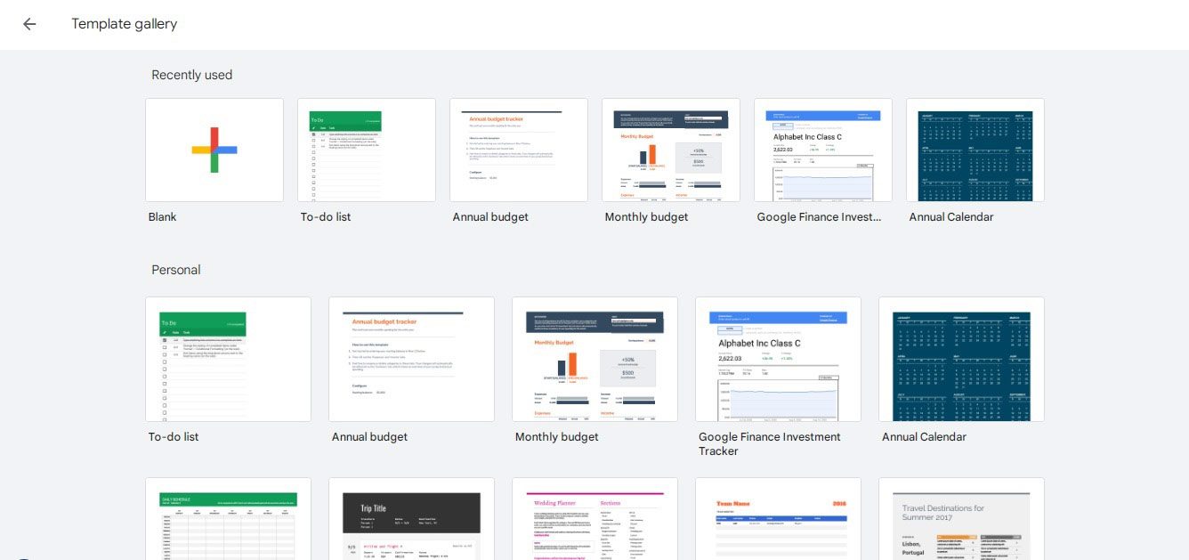
In the new screen, by clicking on the Template Gallery option, you will be faced with a list of preset sheets with different purposes. These pages are divided into Personal, Work, Project Management, and Education categories. The most used are the To-do List, Annual Budget, and Monthly Cost. However, we will work with the Blank option to teach how to work with Google Sheets. A blank page that you can customize to your liking.

You can see the list of your sheets on the main page of Google Sheets. These sheets are listed by their ownership. In front of each page, you can also see when and by whom they were last opened. You can also delete or rename them by clicking on the three-dot menu. Click on the Blank option to enter the main steps of Google Sheet training.

Creating a new page in Google Sheets

 

 

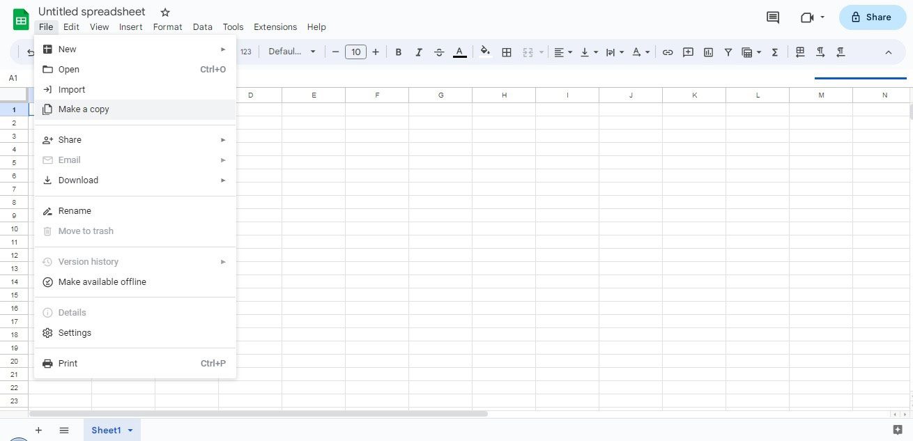
You can see its title at the top of the blank page, which you can change by clicking on it. In raw form, your sheet name is Untitled Spreadsheet. There are different menus under the title. We will work with these menus in the following parts of the article. But at this stage, it is necessary to get acquainted with the most crucial menu, File. The most important options in this menu are:

• New: By clicking this option, you can create a new sheet or access other Google Workspace tools such as Document, Presentation, etc.
  Open and Import: By clicking these options, you can upload the Google Sheet file saved on your computer drive or other files created in Google Sheet or shared with you. Google Sheets also supports Excel, PDF, photo, xlsx, etc. formats.
• Make a Copy: By clicking on this option, you can create a sheet similar to the one you are working on.
• Download as; Click this option to save your File in different formats such as Excel, PDF, and HTML.
• Version History: By clicking on this option, you can view previous versions of your File and, if necessary, restore. This option is especially suitable for projects where different people work simultaneously.
• Make Available Offline: You can make your File available offline by clicking on this option. Before that, however, you must have downloaded and installed the Docs Offline Chrome extension.

After creating your page, you can enter your data in the desired cells. Columns are marked with letters, and rows with numbers. By clicking on each cell, you can enter the data inside it in the upper bar and front of the two fx letters.

• 7 Best JPG To PDF Converter Software For Windows?

 

toolbar: The most crucial step in learning Google Sheets

 

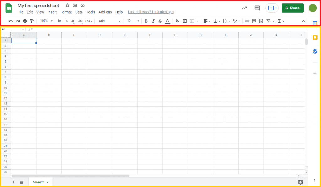
Your main tools when working with Google Sheets are located in the Toolbar. Like many software, this bar can be seen at the top of the screen; ignoring the obvious options such as print, zoom, font, and writing facilities, etc., the most important of these tools from left to right are:

• Undo and Rech move the File to a stage before and after the last change.
• Paint Format applies the format of one section or cell to another area or compartment. The desired configuration can be a formula, font, text, etc.
• The format section that we see after the zoom option. In this section, we have options such as money ($), percentage (%), decimal numbers, and other formats such as date (Date), time (Duration), financial (Financial), and so on.
• The Insert and Filter section, which we see after the writing format section and the rotation tool. In this section, we can enter links, filters, comments, charts, formulas, etc.
• Sort section where we can adjust the direction of the entire Sheet or cells from right to left or vice versa.
• It should be noted that many toolbar features are available in the Edit, View, Insert, Format, and Tools menus and through right-click or shortcut keys.

File sharing in Google Sheets

 

 

One of the most essential topics of Google Sheet training is the software’s features for file sharing and determining its access level. Before that, it is necessary to mention that your data is automatically saved in Google Drive. So you don’t need to use Ctrl + S to save or worry about your data not being saved.

After you’ve created your File by filling in the cells and applying settings, you can share it with multiple people. For this purpose, you need to click on the dummy and + icon in the upper right corner of the image and follow the following steps:

• Specify the name of your File and click the Save button.
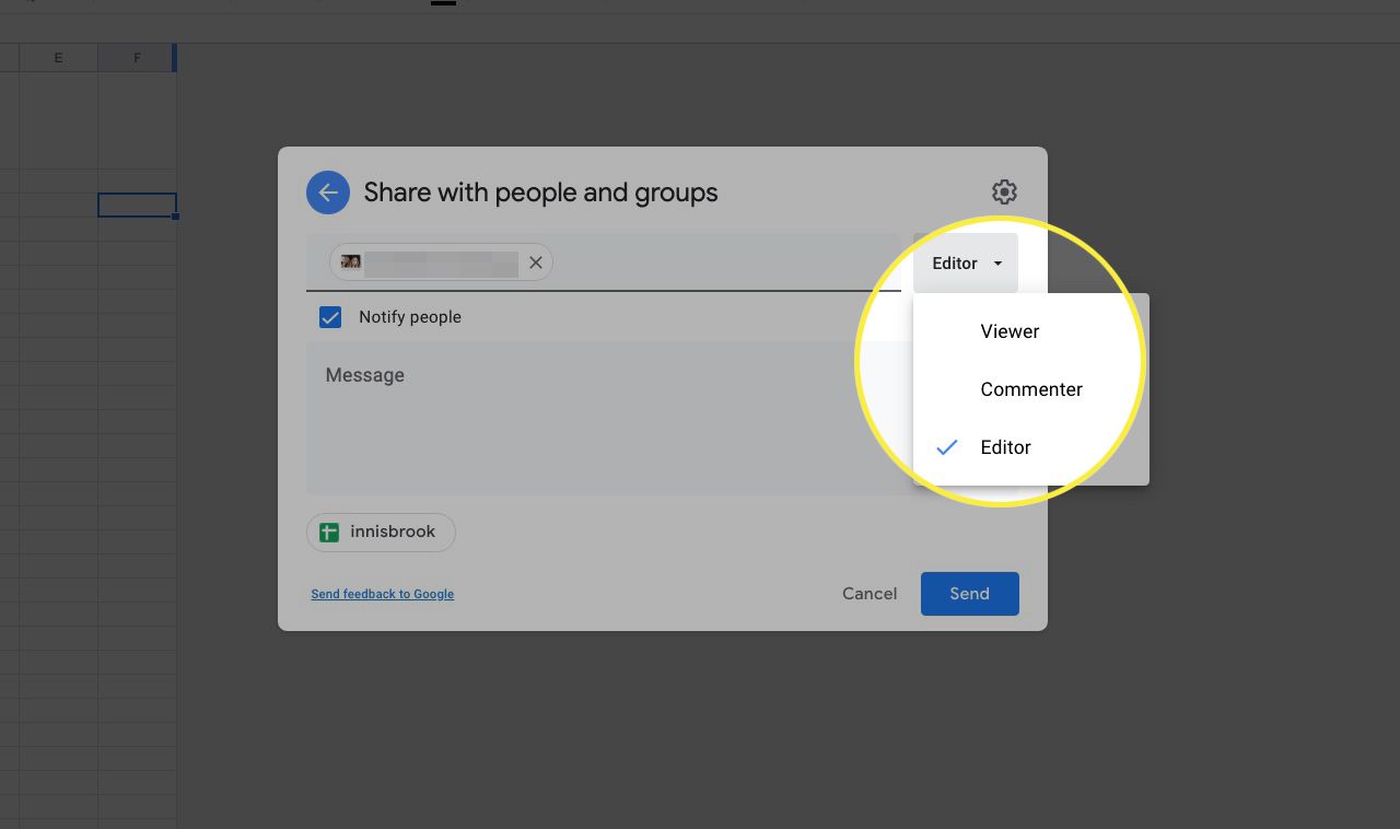
• In the new window, enter the email of the people you want to have access to the File, and for each, choose one of the access levels: Editor, Commenter, or Viewer.
• By ticking the Notify People checkbox, they will be notified via email that your File has been shared with them. You can also write an explanatory text for them in the box below. In the left corner of the box, you can also click on the link symbol to save the web file link to your clipboard.
• By clicking the Send option, the desired access will be granted.
• In the Share window, you can see the list of people with whom the File has been shared. Each person’s access level is also evident. As the File owner, you can change or delete this level.
• You can even transfer ownership of the File to him by clicking Transfer Ownership.

Data protection in Google Sheets

 

 

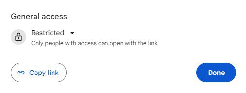
In the lower half of the Share window, which we explained in the previous section, and before specifying people, you can select the level of public access to the File from the General Access section. By clicking on this section, you will be faced with the following two options:

• Restricted. will show the File only to people it has been shared with.
• Anyone With the Link. Which will offer the File to anyone who has a link to it.

 

 

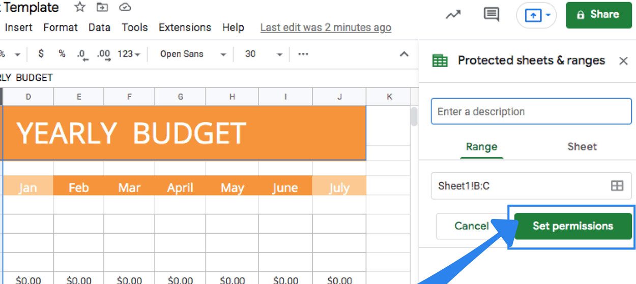
One of the most essential topics of Google Sheet training is limiting the access and viewing of information for other people to the extent of the type of data and part of the Sheet. In other words, you can determine what information each person accessing the File can see. To use this possibility, follow the path below:

• Go to the Data menu at the top of the screen
• Select the Protected Sheets and Ranges option
• Select Range (to hide a p: art of the Sheet) or Sheet (to hide the entire File). By selecting the Sheet option, you can check the Except Certain Cells option and exclude some columns and rows.
• Select the Set Permissions option, and in the opened window, select and set the access levels for this section and notifications. On this page and under the Restrict who can edit this range option, you can repeat the settings of other ranges for this range or Sheet.

Some commonly used data management techniques in Google Sheets

One of the most essential topics in teaching how to use Google Sheets is related to the possibilities of this software for sorting data. For this purpose, filters are the most basic and practical tools. You will especially need these filters if you have a lot of data on a page. They help you decide which data to see and hide more specific data.

Hiding rows and columns

You can hide some of your columns or rows, especially when you don’t want all the columns to be shown to the people with whom the File is shared. To do this, right-click on the desired column or row and then select Hide Column or Hide Row. Doing this, an arrow will appear on the previous and next rows or columns, indicating a hidden row or column between them. As the File owner, you can click these arrows to restore confidential data.

Freeze data

 

 

The next topic in Google Sheets training concerns freezing or fixing data. But before that, we should know why the data is freezing in Google Sheets. When working with a lot of data, it may be necessary to move within the page so that the initial rows and columns are out of sight. Shrinking the screen will also reduce our visibility. Freezing the data we always need while moving on the page helps us not have to return to their original place every time with the mouse. In other words, that row or column will be floating and always in front of your eyes.

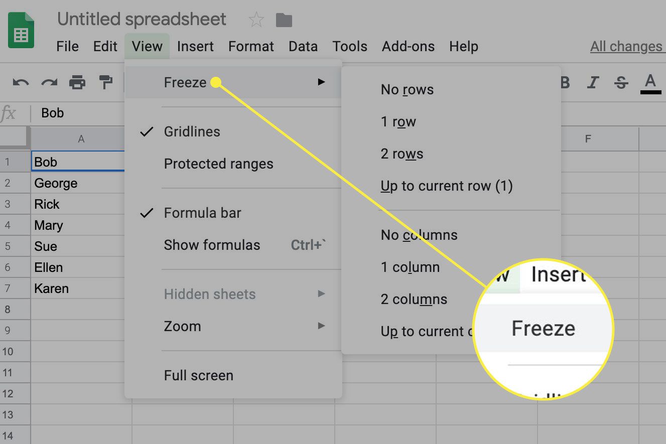
To fix data in Google Sheets, follow the steps below:

• Go to the View menu on the Toolbar.
• Select the Freeze option.
• Choose one of the available options depending on the number of rows or columns you want.

View data based on a filter.

 

 

Another essential technique in Google Sheets training is choosing the type of data displayed based on the formats you’ve already applied to them. By doing this, only the kind of data you are interested in will be shown in each row or column. For example, you can filter only numbers over 500, financial data, specific words, dates, etc. To create a filter, follow the path below:

• Go to the Data menu on the Toolbar.
• Select the Create Filter option.
• You can see that the top and side of the screen turn gray.
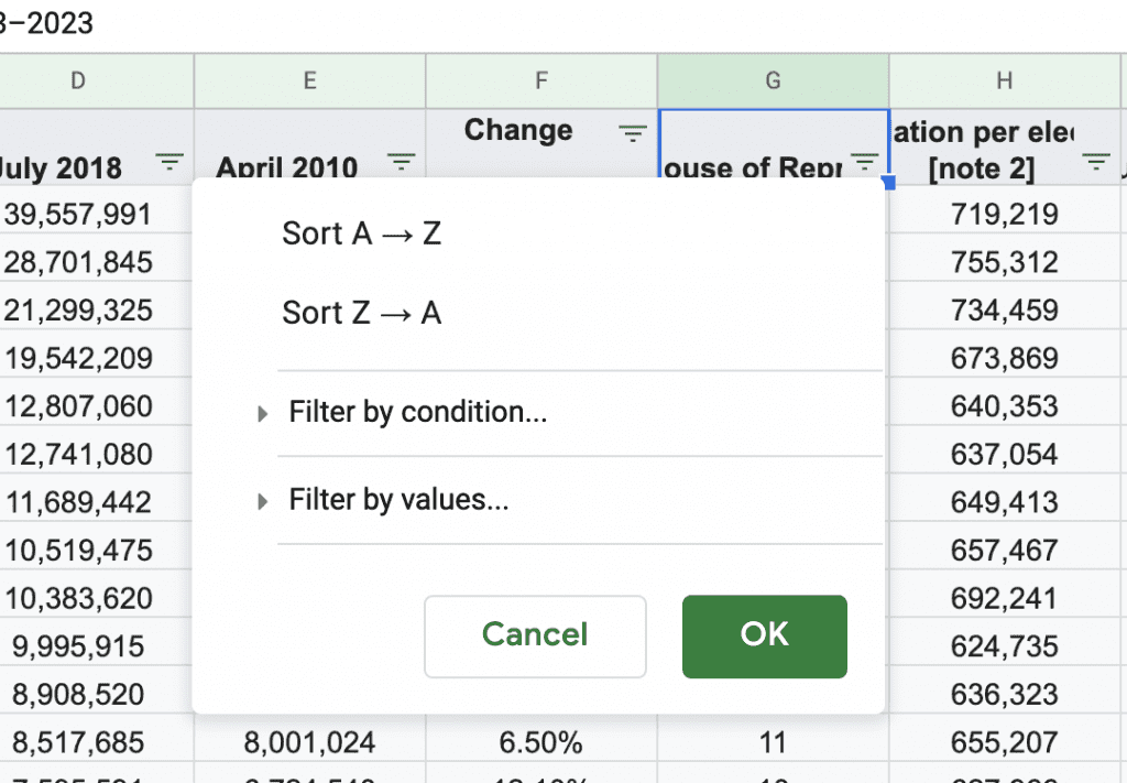
• Click on the three-line icon under the column or next to the row.
• If you want to filter by color, click the Filter By Color option.
• If you want to filter with specific qualitative or quantitative data conditions, click the Filter By Condition option.
• If you want to filter with specific data, click the Filter by Values option.

For example, your most essential filters in the Filter by Condition section are:

• Is Empty; Empty cells
• It is not empty; Non-empty cells
• Text Contains: Cells containing a specific word, letter, or number
• Text Does Not Contain Cells without particular words, letters, or numbers
• Text Starts with Cells, starting with a unique character
• The text ends with Terminating cells with a special character
• The date is Cells containing specific dates
• Date is Before: Cells containing dates before a particular date
• The date is After Cells containing dates after a specific date
• more significant than Cells containing numbers of a certain number
• less than Cells containing numbers more minor than a specified number

Essential Functions in Google Sheets

 

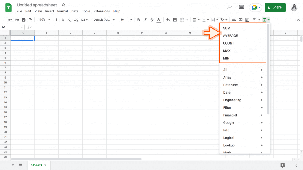
The topic of formula writing is very detailed and usually occupies a large part of every Google Sheet training course. However, you can use some ready-made functions to speed up your work with this software. To use this option, go to the Insert menu and select your mathematical operation or part from the Functions section. These options can also be viewed from the Toolbar by clicking on the Sigma symbol, and the most important ones are:

• SUM or total
• Average
• Max or maximum data
• Min or minimum data
• Countif that counts the number of times the data is repeated based on certain conditions.
• Concatenate, which joins the values of the selected cells together, such as the name of the province and city
• The opposite of concatenate, Split divides the cell values and places them in separate cells.
• Proper, which creates a format for entering data in different cells.

By entering each formula in your cell, you can also write its conditions and range in row and column numbers or manually select the desired cells to be subjected to that function. In addition, you can write your formula in each cell manually.

Resize, add and delete columns and rows in Google Sheets.

 

The contents of your cells may have different lengths. By default, Google Sheets places all data in cells of the same size. Therefore, part of the big data remains hidden and will not be displayed until that cell is clicked. You can move your mouse to the border of two rows or columns until the sign of two parallel lines with an arrow pointing outwards appears. Double-click this symbol to adjust the length of the rows and cells according to the size of the data inside them.

A basic but essential point in Google Sheet training is to add rows and columns in the middle of the page. For this purpose, you must right-click on the desired cell and choose one of the options: Insert 1 row above or Insert 1 column left. This will add a row to the top or a queue to the left of the cell.

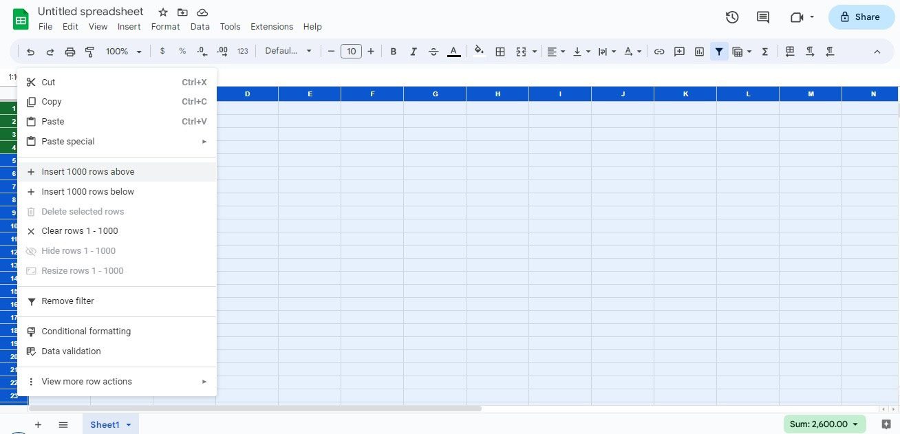
A Google Sheet typically has 1,000 rows. If you need any more rows, as shown in the image above, go to the left corner of your Sheet and the standard cell of the first row and column, and then right-click and click on the option add 1000 rows below or similar.

Commenting on Google Sheets

 

Among the topics related to the collaboration of several people on a project in Google Sheet training are comments or notes. You can comment on each cell separately so the reader knows the points related to the same cell. In this way, you will not need to assign a separate compartment to your comment. For this purpose, follow the steps below:

• Please select the desired cell and right-click on it
• Click on the Comment option.
• Type your desired note and click on the Comment option. You can also tag someone in your comment through their email.

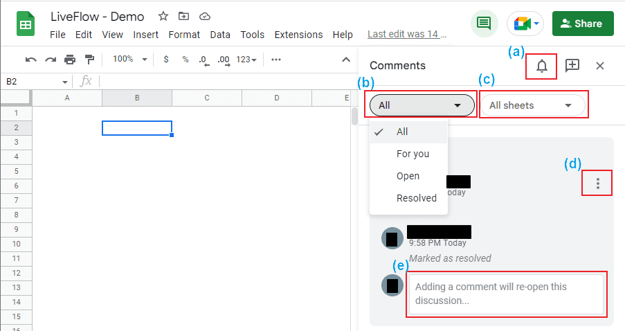
To see all the comments placed on the Sheet, click on the comment icon next to the Call icon, which is in the shape of a camera, on the upper right side of the page. By clicking on each comment, its location in the Sheet will be shown. You can discuss the same cell from here.

Drawing a diagram in Google Sheets

 

One of the advanced topics in Google Sheet training is drawing a diagram. This skill ranges from simple to very complex graphs. In this section, we describe the steps of drawing a simple graph as follows:

• Select the cells you want.
• Go to the Insert menu and select the Chart option.
• Select the Chart Editor tool.
• Choose your chart type from the Column Chart section
• Set other details such as date range.

Here are a few additional tips about working with Google Sheets

At the end of this article, it is necessary to remind you that many of the shortcut keys of Google Sheets and Excel are similar. You can also add a new sheet inside your Sheet by clicking the + option at the bottom of each page in the left corner. In this way, you will have a multi-sheet sheet. Of course, teaching Google Sheets entirely in one article is impossible. The more you master the basic steps of working with this software, the more training you need, which you can find in various Internet sources. What do you think about Google Sheets? Do you prefer this software to Excel?