


Learning R and RStudio is a powerful way to perform data analysis, statistical Modeling, visualization, and more.
R is a programming language and environment designed for statistical computing, while RStudio is an integrated development environment (IDE) that enhances R’s usability with coding, debugging, and visualization tools.
This comprehensive guide will teach you the fundamentals of R programming and how to use RStudio effectively. It covers installation, basic syntax, data manipulation, visualization, and best practices. It’s designed for beginners but includes intermediate concepts to build a strong foundation.

Part 1: Getting Started with R and RStudio

What is R?
- R is an open-source programming language optimized for statistical analysis, data visualization, and machine learning.
- Strengths: Extensive statistical packages, vibrant community, and cross-platform compatibility.
- Use cases: Data analysis, predictive Modeling, scientific research, and reporting.
What is RStudio?
- RStudio is an IDE that provides a user-friendly interface for writing, running, and managing R code.
- Features: Code editor, Console, environment viewer, plotting window, package manager, and support for R Markdown.
- Benefits: Streamlines workflows, supports version control, and enhances productivity.
Step 1: Installation
- Install R:
- Windows/Mac:
- Visit CRAN (Comprehensive R Archive Network).
- Download the latest version of R for your operating system (e.g., R 4.4.1 as of 2025).
- Run the installer and follow the prompts (accept default settings for beginners).
- Linux:
- Use your package manager (e.g., sudo apt install r-base for Ubuntu).
- Windows/Mac:
- Install RStudio:
- Download RStudio Desktop (free version) from posit.co.
- Choose the version for your OS and install it after R (R must be installed first).
- Verify installation by launching RStudio; it should detect R automatically.
- Optional Tools:
- Install Git for version control (git-scm.com).
- Install a LaTeX distribution (e.g., TinyTeX) to render R Markdown documents with equations.
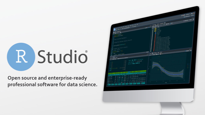
Step 2: Exploring Interface
When you open RStudio, you’ll see four main panes:
- Script Editor (Top Left): Write and save R scripts (.R files) here.
- Console (Bottom Left): Run commands and view output. Type commands directly or run them from scripts.
- Environment/History (Top Right): View loaded datasets, variables, and command history.
- Plots/Packages/Help (Bottom Right): Display visualizations, manage packages, and access documentation.
Tips:
- Customize the layout via View > Panes > Pane Layout.
- Use the Console for quick tests and the Script Editor for reusable code.
- Save scripts frequently to avoid losing work.
Part 2: R Programming Basics
1. Basic Syntax and Operations
R is case-sensitive and uses <- or = for assignment. You can type commands in the Console or save them in a script.
Arithmetic Operations
# Basic math

5 + 3  # Output: 8

10 * 2  # Output: 20

15 / 3  # Output: 5

2^3     # Output: 8 (exponentiation)
Variables
# Assign values to variables

x <- 10

y = 20  # Alternative assignment

z <- x + y

print(z)  # Output: 30
Comments
# Single-line comment

# This is ignored by R
Data Types
- Numeric: 3.14, 42
- Character: “Hello, ‘orld’
- Logical: TRUE, FALSE
- Factors: Categorical data (e.g., “Male”, “Female”)
- Vectors: Collections of similar-type elements
# Create a vector

numbers <- c(1, 2, 3, 4)

names <- c("Alice", "Bob")

logical <- c(TRUE, FALSE)
2. Data Structures
R supports several data structures for storing and manipulating data.
Vectors
- Single-dimensional collections of the same type.
# Create and manipulate vectors

scores <- c(85, 90, 95)

mean(scores)  # Output: 90

scores[1]     # Access first element: 85
Matrices
- Two-dimensional arrays of the same type.
# Create a 2x3 matrix

matrix1 <- matrix(1:6, nrow=2, ncol=3)

print(matrix1)

# Output:

#      [,1] [,2] [,3]

# [1,]    1    3    5

# [2,]    2    4    6
Data Frames
- Tables with rows and columns, like spreadsheets. Columns can have different types.
# Create a data frame

df <- data.frame(

name = c("Alice", "Bob", "Cathy"),

age = c(25, 30, 28),

score = c(85, 90, 95)

)

print(df)

# Output:

#    name age score

# 1 Alice  25    85

# 2   Bob  30    90

# 3 Cathy  28    95
Lists
- Collections of different types of objects.
# Create a list

my_list <- list(name="Alice", age=25, scores=c(85, 90))

print(my_list)
3. Control Structures
Control structures manage the flow of execution.
Conditionals
# If-else statement

x <- 10

if (x > 5) {

print("x is greater than 5")

} else {

print("x is 5 or less")

}
Loops
- For Loop:
for (i in 1:5) {

print(i)

}

# Output: 1, 2, 3, 4, 5- While Loop:
count <- 1

while (count <= 5) {

print(count)

count <- count + 1

}
4. Functions
Functions encapsulate reusable code.
# Define a function

square <- function(x) {

return(x * x)

}

square(4)  # Output: 16
Built-in Functions:
- mean(), sum(), length(), str() (displays object structure)
- Example:
numbers <- c(1, 2, 3, 4)

mean(numbers)  # Output: 2.5
Part 3: Working with Data in R
1. Importing Data
R supports importing data from various sources.
CSV Files
# Read a CSV file

data <- read.csv("path/to/file.csv")

# View first few rows

head(data)
Excel Files
Requires the readxl package.
# Install and load readxl

install.packages("readxl")

library(readxl)

data <- read_excel("path/to/file.xlsx")
Built-in Datasets
R includes sample datasets for practice.
data(mtcars)  # Load the mtcars dataset

head(mtcars)  # View first 6 rows
2. Data Manipulation with dplyr
The dplyr package (part of the tidyverse) simplifies data manipulation.
Install tidyverse
install.packages("tidyverse")

library(tidyverse)
Key dplyr Functions
- Filter: Select rows based on conditions.
# Filter cars with mpg > 20

filtered <- filter(mtcars, mpg > 20)- Select: Choose specific columns.
# Select mpg and hp columns

selected <- select(mtcars, mpg, hp)- Mutate: Create new columns.
# Create a new column: weight in tons

mutated <- mutate(mtcars, wt_tons = wt / 2)- Group by and summarize: Aggregate data.
# Average mpg by number of cylinders

summary <- mtcars %>%

group_by(cyl) %>%

summarize(avg_mpg = mean(mpg))Note: The %>% (pipe operator) passes the result of one function to the next.
3. Handling Missing Data
# Check for missing values

sum(is.na(data))

# Remove rows with missing values

data_clean <- na.omit(data)
Part 4: Data Visualization with ggplot2
The ggplot2 package (part of tidyverse) creates customizable visualizations.
Basic Plot
# Scatter plot of mpg vs. horsepower

ggplot(data = mtcars, aes(x = hp, y = mpg)) +

geom_point() +

labs(title = "MPG vs. Horsepower", x = "Horsepower", y = "MPG")
Customizations
- Add Colors:
ggplot(data = mtcars, aes(x = hp, y = mpg, color = as.factor(cyl))) +

geom_point()- Add Regression Line:
ggplot(data = mtcars, aes(x = hp, y = mpg)) +

geom_point() +

geom_smooth(method = "lm") # Linear model- Facets (subplots):
ggplot(data = mtcars, aes(x = hp, y = mpg)) +

geom_point() +

facet_wrap(~ cyl)
Part 5: Using RStudio Effectively
1. Writing Scripts
- Create a new script: File > New File > R Script.
- Write code in the editor and run lines by:
- Highlighting and pressing Ctrl+Enter (Windows) or Cmd+Enter (Mac).
- Clicking the “Run” button.
- Save scripts with the. Rextension.
2. R Markdown
R Markdown creates dynamic documents combining code, output, and text.
- Create a new R Markdown file: File > New File > R Markdown.
- Write code in code chunks:
```{r}

summary(mtcars)- Knit to HTML/PDF/Word: Click the “Knit” button.
- Install TinyTeX for PDF output:
```R
install.packages("tinytex")
tinytex::install_tinytex()3. Package Management
- Install Packages:
install.packages("package_name")- Load Packages:
library(package_name)- Update Packages:
update.packages()- Use RStudio’s Packages pane to browse and install.
4. Debugging
- Error Messages: Read errors in the Console carefully. Common issues:
- Missing packages: Install the required package.
- Syntax errors: Check for missing parentheses or commas.
- Debugging Tools:
- Use traceback() to see where an error occurred.
- Set breakpoints in RStudio by clicking the left margin of a script.
5. Version Control with Git
- Enable Git in RStudio: Tools > Global Options > Git/SVN.
- Initialize a repository: File > New Project > Version Control > Git.
- Commit and push changes using the Git pane.
Part 6: Intermediate Concepts
1. Writing Efficient Code
- Vectorization: Avoid loops where possible; use vectorized operations.
# Instead of:

result <- c()

for (i in 1:5) {

result[i] <- i^2

}

# Use:

result <- (1:5)^2- Apply Functions:
# Apply a function to each column

col_means <- sapply(mtcars, mean)
2. Statistical Modeling
- Linear Regression:
model <- lm(mpg ~ hp + wt, data = mtcars)

summary(model)- Predictive Modeling (requires caret):
install.packages("caret")

library(caret)

# Example: Train a model

train(mpg ~ ., data = mtcars, method = "lm")
3. Working with APIs
- Use httr to fetch data from APIs.
install.packages("httr")

library(httr)

response <- GET("https://api.example.com/data")

data <- content(response, "parsed")
4. Shiny Apps
Create interactive web apps with the Shiny package.
install.packages("shiny")

library(shiny)

ui <- fluidPage(

sliderInput("num", "Choose a number", 1, 100, 50),

textOutput("square")

)

server <- function(input, output) {

output$square <- renderText({ input$num^2 })

}

shinyApp(ui, server)
Part 7: Best Practices and Resources
Best Practices
- Organize Code:
- Use comments to explain logic.
- Break the code into functions for reusability.
- Save scripts in a project directory (File > New Project).
- Reproducible Research:
- Use R Markdown for reports.
- Set a random seed for reproducibility: set. seed(123).
- Performance:
- Use data. Table or dplyr for large datasets.
- Avoid unnecessary copying of objects.
- Community Standards:
- Follow tidyverse style guide (style.tidyverse.org).
- Share code via GitHub or RPubs.
Troubleshooting
- Package Conflicts: Load packages in the correct order or use:: (e.g., dplyr::filter).
- Memory Issues: Clear the environment with rm(list = ls()) or use gc() for garbage collection.
- Installation Errors: Ensure R and RStudio are up to date. Check CRAN mirrors.
Learning Resources
- Books:
- R for Data Science by Hadley Wickham (free online: r4ds.had.co.nz).
- Hands-On Programming with R by Garrett Grolemund.
- Online Courses:
- DataCamp: Interactive R tutorials.
- Coursera: “Data Science” specialization by Johns Hopkins.
- Communities:
- Stack Overflow (tag: [r]).
- RStudio Community (community.rstudio.com).
- X posts: Search for #RStats for tips and updates.
- Documentation:
- Use ?function_name or help(function_name) in RStudio.
- CRAN package vignettes.
Practice Exercises
- Basic:
- Create a vector of your favorite numbers and calculate their mean and standard deviation.
- Build a data frame with the names and ages of 5 friends.
- Data Manipulation:
- Load the mtcars dataset and filter cars with horsepower > 150.
- Create a new column for miles per gallon per cylinder.
- Visualization:
- Plot a histogram of mtcars$mpg using ggplot2.
- Create a scatter plot of wt vs. mpg, colored by cyl.
- R Markdown:
- Write an R Markdown document summarizing the mtcars dataset with a plot and knit it to HTML.
Conclusion
R and RStudio form a robust ecosystem for data analysis and visualization. You can handle a wide range of data tasks by mastering basic syntax, data structures, dplyr, ggplot2, and RStudio’s features like R Markdown and package management.
Start with small scripts, explore built-in datasets, and gradually tackle intermediate topics like Modeling and Shiny apps. Use the recommended resources and practice regularly to build proficiency.
FAQ
Do I need prior programming experience to follow this 40-minute training?
No — the guide is designed for beginners and assumes no prior coding experience.
Will I be able to analyze real-world datasets after completing this training?
Yes — you’ll learn the basics of importing data and generating simple plots, which serve as a foundation for deeper data analysis.
What should I have installed before beginning the training?
Make sure you have both R and RStudio installed on your computer so you can follow along with the interface and code examples.