Deep Neural Networks Are One Of The Most Widely Used Areas Of Artificial Intelligence That Provide Practical Capabilities To Organizations. 

Keras Deep Learning Library, the use of deep networks goes beyond the everyday needs of ordinary companies, and, to be more precise, they are used for professional purposes.

One of the most powerful libraries available to users to build and build a neural network is the Keras library, open to Python developers.

In this article, we want to show you how to work with this library.

How to train an artificial neural network?

Typically, training an artificial neural network consists of the following seven steps:

1. The weights are randomly initialized with values ​​close to zero but non-zero.

2. Data set observations are given to the input layer.

3. Forward propagation (left to right): The nerve cells are activated, and the predicted values ​​are obtained.

4. The predicted computer results are compared with the actual values, ​​and the error rate is calculated.

5. Backward (from right to left): Weights are adjusted.

6. Steps 1 to 5 are repeated.

7. A course (Epoch) is obtained when the whole training is passed through the neural network. A course (Epoch) is obtained.

Business issue

Now it’s time to explore real-world business issues using the Keras neural network and Python library. Suppose we have an insurance company that has a collection of claims from its customers. The insurance company is now asking a data mining expert to help them predict which claims are valid and fraudulent. It allows the insurance company to save millions of dollars annually.

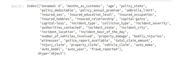
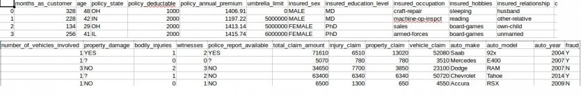
This model of problems is grouped into categorization problems. The columns of this data set that are related to the claims of the insurance company’s customers are shown in the following image:

 

Data processing

Like most business issues, aggregated data is not ready for analysis. Therefore, the data mining specialist must make them understandable to the algorithm. According to the data set, it was evident that there are several columns with the categorical data types.

For the deep learning algorithm to understand the data, the data must convert to zeros and ones. Another issue we need to address is that the data set should provide to the model in a NumPy array. For Using the following code snippet, the necessary packages are entered into the program, after which the data set of the insurance company is loaded.

import pandas as PD

import NumPy as np

df = PD.read_csv(‘Datasets/claims/insurance_claims.csv’)

Subsequently, the class columns are converted to virtual variables (Dummy Variables).

feats = [‘policy_state’,’insured_sex’,’insured_education_level’,’insured_occupation’,’insured_hobbies’,’insured_relationship’,’collision_type’,’incident_severity’,’authorities_contacted’,’incident_state’,’incident_city’,’incident_location’,’property_damage’,’police_report_available’,’auto_make’,’auto_model’,’fraud_reported’,’incident_type’]

df_final = PD.get_dummies(df,columns=feats,drop_first=True)

The above command uses drop_first = True to prevent the Trap problem from appearing about variables. For example, if d, c, b, a are classes, d can be omitted as an apparent variable because if something was not inside b, a, and c, it exists in d. It is called multicollinearity. The train_test_split of the Psychitlern library is now used to divide data into training and test categories.

from sklearn.model_selection import train_test_split

At this point, you should make sure that the column is removed when forecasting so as not to cause an overflow problem in the training and testing suite. Note, however, that you should not use the same data set to train and test the model. To get the NumPy array developed at the end of the data set (values). The above approach is a solution that accepts the data learning model (Deep Learning). This step is important because the machine learning model built in this article agrees with the data in an array.

X = df_final.drop([‘fraud_reported_Y’,’policy_csl’,’policy_bind_date’,’incident_date’],axis=1).values

y = df_final [‘fraud_reported_Y’]. values

The data is then divided into training and experimental sets. 0.7 of the data is used for training and 0.3 for testing.

X_train, X_test, y_train, y_test = train_test_split(X, y, test_size=0.3)

Next, the data set must be scaled using the Sklearn Library StandardScaler. Due to the large number of computations performed in deep learning, feature scaling is essential. Scaling characterizes the range of independent variables.

from sklearn.preprocessing import StandardScaler

sc = StandardScaler()

X_train = sc.fit_transform(X_train)

X_test = sc.transform(X_test)

How to build an artificial neural network

To build an artificial neural network, the first thing you need to do is import the Keras library. Cross uses TensorFlow as a backend by default.

hard import

Next, you need to enter some Keras modules. The Sequential module is used to initialize the deep neural network, and the Dense module is used to build the layers of the artificial neural network.

From Keras. Models import Sequential

from Keras. layers import Dense

Next, you need to initialize the deep neural network by making a sequential instance. The Sequential function initializes a linear stack of layers to add layers using the Dense module in the future.

classifier = Sequential()

Add input layer (first hidden layer)

The add method is used to add different layers to the neural network. The first parameter is the number of nodes that the user has to add to this layer. There is no set rule for calculating how many nodes should add. Of course, most experts choose the number of nodes equal to the average number of nodes in the input layer and the number of nodes in the output layer.

For example, if there are five independent variables and one output, their sum is calculated and divided by two, equal to three. In addition, it can test with a method called Parameter Tuning.

The second parameter, kernel_initializer, is a function for initializing weights. In this case, the Uniform Distribution ensures that the consequences are small numbers close to zero.

The following parameter is the Activation Function. In the above example, the rectifier function, summarized as relu in the activation function, is used. This function is often used for the hidden layer in the deep neural network.

The final parameter is called input_dim, which is the number of nodes hidden in the layer. This parameter indicates the number of independent variables.

classifier.add(

Dense(3, kernel_initializer = ‘uniform’,

activation = ‘relax, input_dim=5))

Add the second hidden layer

Adding the second hidden layer is similar to the previous case.

classsifier.add(

Dense(3, kernel_initializer = ‘uniform’,

activation = ‘reread’))

There is no need to specify the input_dim parameter here because it is established in the first hidden layer. This variable is defined in the first hidden layer to allow the coating to know how many input nodes to expect. The deep neural network knows how many input nodes to expect in the second hidden layer, so we should not look for repetition.

Add output layer

classifier.add(

Dense(1, kernel_initializer = ‘uniform’,

activation = ‘sigmoid’))

The first parameter must change because we expect a node in the output node. Because in this case, the purpose is to determine whether a claim is fraudulent or not. It is done using the Sigmoid Activation Function. If the issue is categorized and has more than two classes, two things must change. Change the first parameter to 3 and the activation function to softmax. Softmax is a sigmoid function applied to an independent variable with more than two categories.

Compile artificial neural network

classifier.compile(optimizer= ‘adam’,

loss = ‘binary_crossentropy’,

metrics = [‘accuracy’])

Compiling means applying a Stochastic Gradient Descent to the entire neural network. The first parameter is an algorithm for obtaining the optimal set of weights in the neural network. There are many different types of these parameters. One of the most effective algorithms for this is Adam. The second parameter of the loss function within the random gradient algorithm is random. Since binaries are binary, the binary_crossentropy process is used.

Otherwise, categorical_crossentopy was used. The final argument is the criterion used to evaluate the model. In the above example, accuracy is used to assess the model.

Fitting a deep neural network to a training set

classifier.fit(X_train, y_train, batch_size = 10, epochs = 100)

X_train shows the independent variables used to train the neural network, and y_train describes the column to be predicted. Epochs represent the number of times a complete data set is routed to an artificial neural network. Batch_size is the number of observations based on which weights are updated.

Prediction using the training set

y_pred = classifier.predict(X_test)

This code indicates that a claim may be fraudulent. Then, a 50% threshold for classifying a claim is considered fraud. It means that any claim with a probability of half a percent or more is considered fraud.

y_pred = (y_pred> 0.5)

In this case, the insurance company can pursue claims that are not suspicious and has more time to evaluate the claims that have been marked as fraud.

Examination of the perturbation matrix

from sklearn.metrics import confusion_matrix

cm = confusion_matrix(y_test, y_pred)

The Confusion Matrix can be considered a form that out of 2000 observations, 175 + 1550 comments are correctly predicted. At the same time, 45 + 230 cases have been expected incorrectly. Accuracy can be calculated by dividing the number of correct predictions by the total projections. This example is 2000 / (175 + 1550), which is equal to 86% accuracy.

Make a prediction

Suppose an insurance company claims an expert. They want to know if this claim is fraudulent. How can such an issue be understood?

new_pred = classifier.predict(sc.transform(np.array([[a,b,c,d]])))

In the code above, d, c, b, a represent the properties that exist.

new_pred = (new_prediction > 0.5)

Since the classifier expects NumPy arrays as input, a single view must be converted to a NumPy array, and a standard scaler is used to scale it.

Evaluation of artificial neural network designed.

After training the model once or twice, it can seem that different accuracy is obtained. So you can’t be sure which ones are right. It raises the issue of Bias Variance Trade-Off. Therefore, after being caught several times, we should teach a correct model without much accuracy variance. It is to solve this problem, cross-validation of K-fold with K equal to 10 is used.

The above approach causes the training set to be set to 10 fold. Next, the model is trained on 9 folds and tested on the remaining folds. Since there are 10 folds, we try to do this recursively through 10 combinations. Each iteration is correct. In the following, the average of all accuracy is calculated and used as the model accuracy.

from keras.wrappers.scikit_learn import KerasClassifier

Then, the K-fold cross-validation function is imported from scikit_learn.

from sklearn.model_selection import cross_val_score

KerasClassifier expects one of its arguments to be a function, so it needs to be built into that function. The purpose of this function is to build an artificial neural network architecture.

def make_classifier():

    classifier = Sequential()

    classiifier.add(Dense(3, kernel_initializer = ‘uniform’, activation = ‘relu’, input_dim=5))

    classiifier.add(Dense(3, kernel_initializer = ‘uniform’, activation = ‘relu’))

    classifier.add(Dense(1, kernel_initializer = ‘uniform’, activation = ‘sigmoid’))

    classifier.compile(optimizer= ‘adam’,loss = ‘binary_crossentropy’,metrics = [‘accuracy’])

    return classifier

This function creates the categorizer and returns it for use in the next step. The only thing is to cover the previous deep neural network architecture in the function and restore the categorization. Next, a new categorizer is created using K-fold cross-validation, and the build_fn parameter is passed to it as a function built above.

classifier = KerasClassifier(build_fn = make_classifier,

                            batch_size=10, nb_epoch=100)

The scikit-learn library cross_val_score function is used to apply the K-fold cross-validation function. The estimator is a category created using make_classifier, and n_jobs = -1 allows all available processors. Cv The number of folds and 10 is a common choice—cross_val_score Returns ten of the tenfold tests used in calculations.

accuracies = cross_val_score(estimator = classifier,

                             X = X_train,

                             y = y_train,

                             cv = 10,

                             n_jobs = -1)

The average accuracy is obtained to obtain Relative Accuracies.

mean = accuracies.mean()

To calculate the variance, we do the following:

variance = accuracies.var()

Here we are looking for low variance between accuracy.

Excessive

Overfitting in machine learning occurs when the model learns the details and noise in the data set and thus performs poorly on the test dataset. It occurs when there is a significant difference between the accuracy of the test set and the training set or when there is a high variance when applying K-fold cross-validation.

In artificial neural networks, this problem is addressed through a method called (Dropout Regularization).

Dropout Regularization works by accidentally deactivating some nerve cells in each repetition of training to prevent them from becoming too independent of each other.

from keras.layers import Dropout

classifier = Sequential()

classiifier.add(Dense(3, kernel_initializer = ‘uniform’, activation = ‘relu’, input_dim=5))

# Notice the dropouts

classifier.add(Dropout(rate = 0.1))

classiifier.add(Dense(6, kernel_initializer = ‘uniform’, activation = ‘relu’))

classifier.add(Dropout(rate = 0.1))

classifier.add(Dense(1, kernel_initializer = ‘uniform’, activation = ‘sigmoid’))

classifier.compile(optimizer= ‘adam’,loss = ‘binary_crossentropy’,metrics = [‘accuracy’])

In the example above, dropout can be done after the first output layer and after the second hidden layer. Using a rate of 0.1 means that 1% of the nerve cells will be inactivated in each repetition. It is recommended to work at a rate of 0.1. However, it should never be more than 0.4, as the model will be underfitting.

Parameter setting

Once the desired accuracy is achieved, the parameters can adjust for higher accuracy. Grid Search allows the user to calculate various parameters to get the best parameters. The first step here is to import the GridSearchCV module from sklearn.

from sklearn.model_selection import GridSearchCV

In addition, the make_classifier function needs to be edited as taught below. A new variable called optimizer is created to allow more than one optimizer to be added to the params variable.

def make_classifier(optimizer):

    classifier = Sequential()

    classiifier.add(Dense(6, kernel_initializer = ‘uniform’, activation = ‘relu’, input_dim=11))

    classiifier.add(Dense(6, kernel_initializer = ‘uniform’, activation = ‘relu’))

    classifier.add(Dense(1, kernel_initializer = ‘uniform’, activation = ‘sigmoid’))

    classifier.compile(optimizer= optimizer,loss = ‘binary_crossentropy’,metrics = [‘accuracy’])

    return classifier

Here, the KerasClassifier is still used, but the batch size and number of epochs are not sent, as these are the parameters to be set.

classifier = KerasClassifier(build_fn = make_classifier)

The next step is to create a dictionary with the specified parameters to be set. Here are the batch size, number of cycles, and the optimization function of these parameters. Adam is also used for the optimizer, and a new optimizer called rmsprop is added.

The Keras documentation suggests the use of rmsprop when working with recurrent neural networks. However, it can also use for this artificial neural network to assess its impact on improving outcomes.

params = {

    ‘batch_size’:[20,35],

    ‘nb_epoch’:[150,500],

    ‘Optimizer’:[‘adam’,’rmsprop’]

}

Grid Search is then used to test these parameters. The Grid Search function will read the scoring criteria and the number of k-folds from the parameter estimator.

grid_search = GridSearchCV(estimator=classifier,

                           param_grid=params,

                           scoring=’accuracy’,

                           cv=10)

Like the previous objects, it needs to fit the training dataset.

grid_search = grid_search.fit(X_train,y_train)

The best selection of parameters can be obtained using the best_params from the grid search object. Similarly, best_score is used to get the best score.

best_param = grid_search.best_params_

best_accuracy = grid_search.best_score_

Note that the above process is a bit time-consuming because it searches for the best parameters.